Optimisation
ACTL3143 & ACTL5111 Deep Learning for Actuaries
Patrick Laub
Dense Layers in Matrices
Lecture Outline
Dense Layers in Matrices
Optimisation
Loss and derivatives
Logistic regression
Observations: \mathbf{x}_{i,\bullet} \in \mathbb{R}^{2}.
Target: y_i \in \{0, 1\}.
Predict: \hat{y}_i = \mathbb{P}(Y_i = 1).
The model
For \mathbf{x}_{i,\bullet} = (x_{i,1}, x_{i,2}): z_i = x_{i,1} w_1 + x_{i,2} w_2 + b
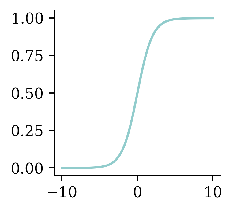
\hat{y}_i = \sigma(z_i) = \frac{1}{1 + \mathrm{e}^{-z_i}} .
Multiple observations
| x_1 | x_2 | y | |
|---|---|---|---|
| 0 | 1 | 2 | 0 |
| 1 | 3 | 4 | 1 |
| 2 | 5 | 6 | 1 |
Let w_1 = 1, w_2 = 2 and b = -10.
Matrix notation
Have \mathbf{X} \in \mathbb{R}^{3 \times 2}.
\mathbf{z} = \mathbf{X} \mathbf{w} + b , \quad \mathbf{a} = \sigma(\mathbf{z})
Using a softmax output
Observations: \mathbf{x}_{i,\bullet} \in \mathbb{R}^{2}. Predict: \hat{y}_{i,j} = \mathbb{P}(Y_i = j).
Target: \mathbf{y}_{i,\bullet} \in \{(1, 0), (0, 1)\}.
The model: For \mathbf{x}_{i,\bullet} = (x_{i,1}, x_{i,2}) \begin{aligned} z_{i,1} &= x_{i,1} w_{1,1} + x_{i,2} w_{2,1} + b_1 , \\ z_{i,2} &= x_{i,1} w_{1,2} + x_{i,2} w_{2,2} + b_2 . \end{aligned}
\begin{aligned} \hat{y}_{i,1} &= \text{Softmax}_1(\mathbf{z}_i) = \frac{\mathrm{e}^{z_{i,1}}}{\mathrm{e}^{z_{i,1}} + \mathrm{e}^{z_{i,2}}} , \\ \hat{y}_{i,2} &= \text{Softmax}_2(\mathbf{z}_i) = \frac{\mathrm{e}^{z_{i,2}}}{\mathrm{e}^{z_{i,1}} + \mathrm{e}^{z_{i,2}}} . \end{aligned}
Multiple observations
Choose:
w_{1,1} = 1, w_{2,1} = 2,
w_{1,2} = 3, w_{2,2} = 4, and
b_1 = -10, b_2 = -20.
Matrix notation
\mathbf{Z} = \mathbf{X} \mathbf{W} + \mathbf{b} , \quad \mathbf{A} = \text{Softmax}(\mathbf{Z}) .
Optimisation
Lecture Outline
Dense Layers in Matrices
Optimisation
Loss and derivatives
Gradient-based learning
In-class demo
Gradient descent pitfalls

Go over all the training data
Called batch gradient descent.
Pick a random training example
Called stochastic gradient descent.
Take a group of training examples
Called mini-batch gradient descent.
Mini-batch gradient descent
Why?
- Because we have to (data is too big to shove it all in a single batch)
- Because it is faster (lots of quick noisy steps takes longer than a few slow super accurate steps)
- The noise helps us jump out of local minima
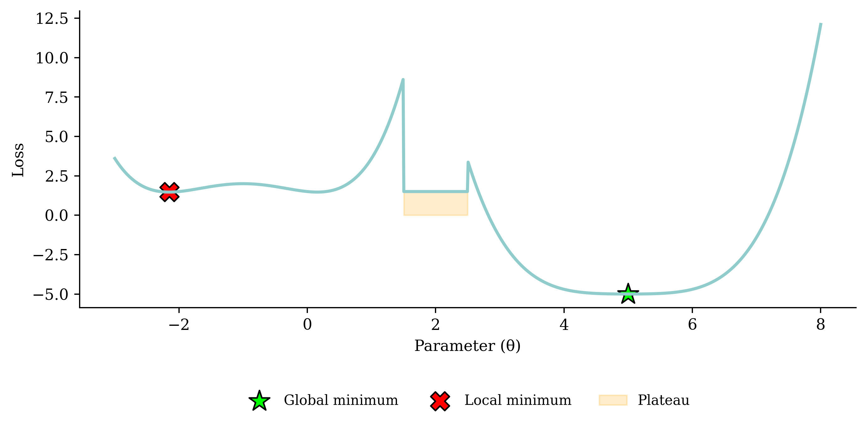
Noisy gradient means we might jump out of a local minimum.
Learning rates
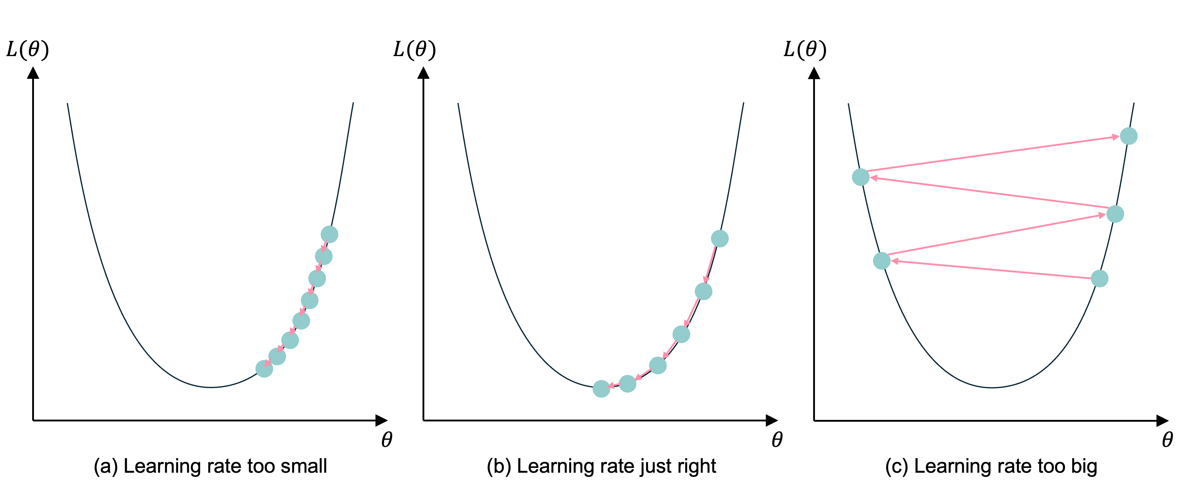
Gradient descent with different learning rates
Source: Melissa Renard (2025), adapted from Jeremy Jordan (2018), Setting the learning rate of your neural network.
Learning rates #2
Source: Matt Henderson (2021), Twitter post
Learning rate schedule
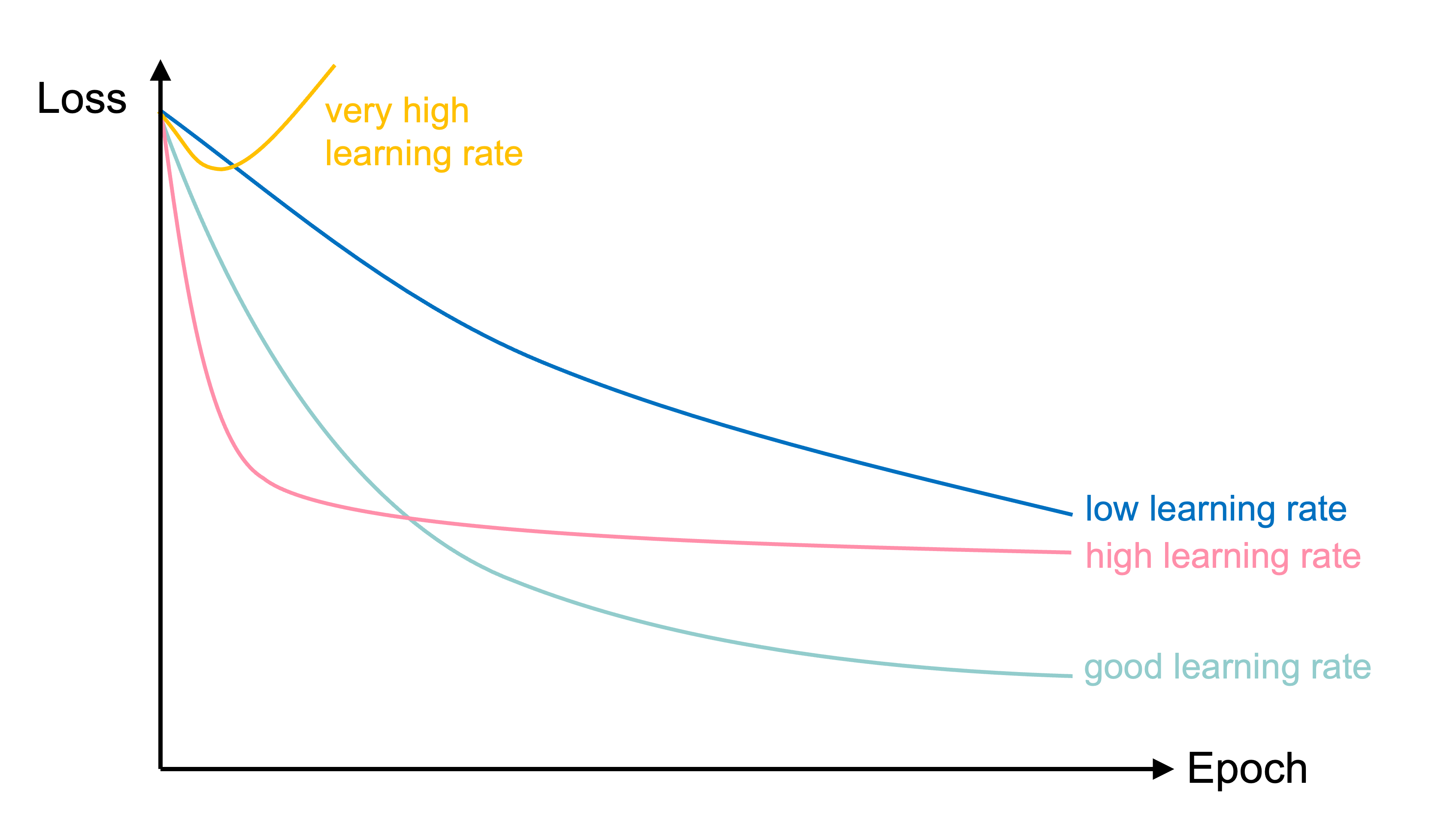
Learning curves for various learning rates
In training the learning rate may be tweaked manually.
Source: Melissa Renard (2025), adapted from Deep Learning for Computer Vision - Stanford Spring 2025
Loss and derivatives
Lecture Outline
Dense Layers in Matrices
Optimisation
Loss and derivatives
Example: linear regression
\hat{y}(x) = w x + b
For some observation \{ x_i, y_i \}, the squared error loss is
\text{Loss}_i = (\hat{y}(x_i) - y_i)^2
For a batch of the first n observations the MSE loss is
\text{Loss}_{1:n} = \frac{1}{n} \sum_{i=1}^n (\hat{y}(x_i) - y_i)^2
Derivatives
Since \hat{y}(x) = w x + b,
\frac{\partial \hat{y}(x)}{\partial w} = x \text{ and } \frac{\partial \hat{y}(x)}{\partial b} = 1 .
As \text{Loss}_i = (\hat{y}(x_i) - y_i)^2, we know \frac{\partial \text{Loss}_i}{\partial \hat{y}(x_i) } = 2 (\hat{y}(x_i) - y_i) .
Chain rule
\frac{\partial \text{Loss}_i}{\partial \hat{y}(x_i) } = 2 (\hat{y}(x_i) - y_i), \,\, \frac{\partial \hat{y}(x)}{\partial w} = x , \, \text{ and } \, \frac{\partial \hat{y}(x)}{\partial b} = 1 .
Putting this together, we have
\frac{\partial \text{Loss}_i}{\partial w} = \frac{\partial \text{Loss}_i}{\partial \hat{y}(x_i) } \times \frac{\partial \hat{y}(x_i)}{\partial w} = 2 (\hat{y}(x_i) - y_i) \, x_i
and \frac{\partial \text{Loss}_i}{\partial b} = \frac{\partial \text{Loss}_i}{\partial \hat{y}(x_i) } \times \frac{\partial \hat{y}(x_i)}{\partial b} = 2 (\hat{y}(x_i) - y_i) .
We need non-zero derivatives
This is why can’t use accuracy as the loss function for classification.
Also why we can have the dead ReLU problem.
Stochastic gradient descent (SGD)
Start with \boldsymbol{\theta}_0 = (w, b)^\top = (0, 0)^\top.
Randomly pick i=5, say x_i = 5 and y_i = 5.
\hat{y}(x_i) = 0 \times 5 + 0 = 0 \Rightarrow \text{Loss}_i = (0 - 5)^2 = 25.
The partial derivatives are \begin{aligned} \frac{\partial \text{Loss}_i}{\partial w} &= 2 (\hat{y}(x_i) - y_i) \, x_i = 2 \cdot (0 - 5) \cdot 5 = -50, \text{ and} \\ \frac{\partial \text{Loss}_i}{\partial b} &= 2 (0 - 5) = - 10. \end{aligned} The gradient is \nabla \text{Loss}_i = (-50, -10)^\top.
SGD, first iteration
Start with \boldsymbol{\theta}_0 = (w, b)^\top = (0, 0)^\top.
Randomly pick i=5, say x_i = 5 and y_i = 5.
The gradient is \nabla \text{Loss}_i = (-50, -10)^\top.
Use learning rate \eta = 0.01 to update \begin{aligned} \boldsymbol{\theta}_1 &= \boldsymbol{\theta}_0 - \eta \nabla \text{Loss}_i \\ &= \begin{pmatrix} 0 \\ 0 \end{pmatrix} - 0.01 \begin{pmatrix} -50 \\ -10 \end{pmatrix} \\ &= \begin{pmatrix} 0 \\ 0 \end{pmatrix} + \begin{pmatrix} 0.5 \\ 0.1 \end{pmatrix} = \begin{pmatrix} 0.5 \\ 0.1 \end{pmatrix}. \end{aligned}
SGD, second iteration
Start with \boldsymbol{\theta}_1 = (w, b)^\top = (0.5, 0.1)^\top.
Randomly pick i=9, say x_i = 9 and y_i = 17.
The gradient is \nabla \text{Loss}_i = (-223.2, -24.8)^\top.
Use learning rate \eta = 0.01 to update \begin{aligned} \boldsymbol{\theta}_2 &= \boldsymbol{\theta}_1 - \eta \nabla \text{Loss}_i \\ &= \begin{pmatrix} 0.5 \\ 0.1 \end{pmatrix} - 0.01 \begin{pmatrix} -223.2 \\ -24.8 \end{pmatrix} \\ &= \begin{pmatrix} 0.5 \\ 0.1 \end{pmatrix} + \begin{pmatrix} 2.232 \\ 0.248 \end{pmatrix} = \begin{pmatrix} 2.732 \\ 0.348 \end{pmatrix}. \end{aligned}
Batch gradient descent (BGD)
For the first n observations \text{Loss}_{1:n} = \frac{1}{n} \sum_{i=1}^n \text{Loss}_i so
\begin{aligned} \frac{\partial \text{Loss}_{1:n}}{\partial w} &= \frac{1}{n} \sum_{i=1}^n \frac{\partial \text{Loss}_{i}}{\partial w} = \frac{1}{n} \sum_{i=1}^n \frac{\partial \text{Loss}_{i}}{\hat{y}(x_i)} \frac{\partial \hat{y}(x_i)}{\partial w} \\ &= \frac{1}{n} \sum_{i=1}^n 2 (\hat{y}(x_i) - y_i) \, x_i . \end{aligned}
\begin{aligned} \frac{\partial \text{Loss}_{1:n}}{\partial b} &= \frac{1}{n} \sum_{i=1}^n \frac{\partial \text{Loss}_{i}}{\partial b} = \frac{1}{n} \sum_{i=1}^n \frac{\partial \text{Loss}_{i}}{\hat{y}(x_i)} \frac{\partial \hat{y}(x_i)}{\partial b} \\ &= \frac{1}{n} \sum_{i=1}^n 2 (\hat{y}(x_i) - y_i) . \end{aligned}
BGD, first iteration (\boldsymbol{\theta}_0 = \boldsymbol{0})
| x | y | y_hat | loss | dL/dw | dL/db | |
|---|---|---|---|---|---|---|
| 0 | 1 | 0.99 | 0 | 0.98 | -1.98 | -1.98 |
| 1 | 2 | 3.00 | 0 | 9.02 | -12.02 | -6.01 |
| 2 | 3 | 5.01 | 0 | 25.15 | -30.09 | -10.03 |
So \nabla \text{Loss}_{1:3} is
so with \eta = 0.1 then \boldsymbol{\theta}_1 becomes
BGD, second iteration
| x | y | y_hat | loss | dL/dw | dL/db | |
|---|---|---|---|---|---|---|
| 0 | 1 | 0.99 | 2.07 | 1.17 | 2.16 | 2.16 |
| 1 | 2 | 3.00 | 3.54 | 0.29 | 2.14 | 1.07 |
| 2 | 3 | 5.01 | 5.01 | 0.00 | -0.04 | -0.01 |
So \nabla \text{Loss}_{1:3} is
so with \eta = 0.1 then \boldsymbol{\theta}_2 becomes
Glossary
- batch gradient descent
- batches, batch size
- global minimum, local minimum
- gradient-based learning, hill-climbing
- learning rate, learning rate schedule
- plateau
- stochastic gradient descent
- mini-batch gradient descent
![]()