Computer Vision
ACTL3143 & ACTL5111 Deep Learning for Actuaries
Shapes of data
Illustration of tensors of different rank.
Shapes of photos

A photo is a rank 3 tensor.
How we see them
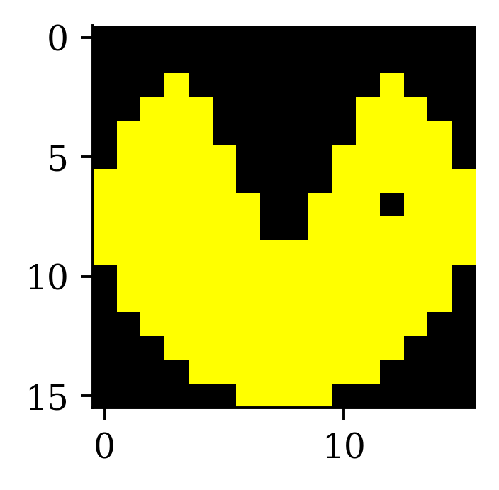
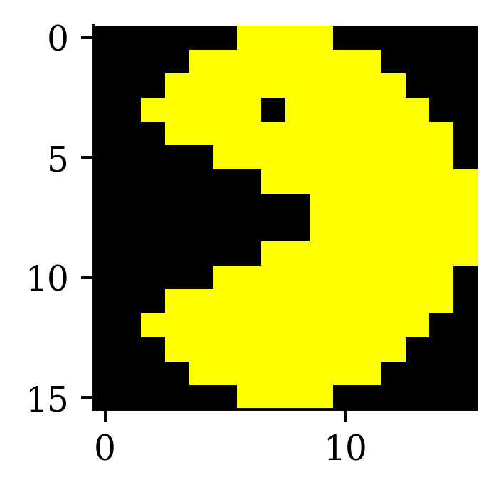
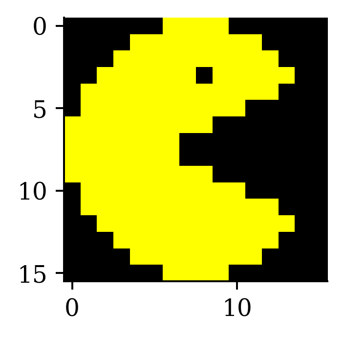
Image editing with kernels
Take a look at https://setosa.io/ev/image-kernels/.
An example of an image kernel in action.
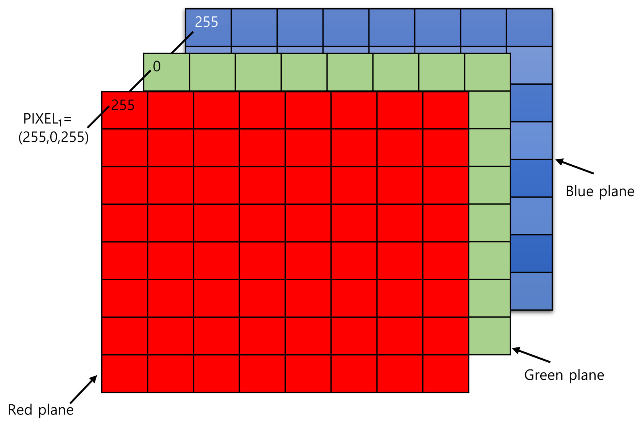
Images are rank 3 tensors
Height, width, and number of channels.
Examples of rank 3 tensors.
Grayscale image has 1 channel. RGB image has 3 channels.
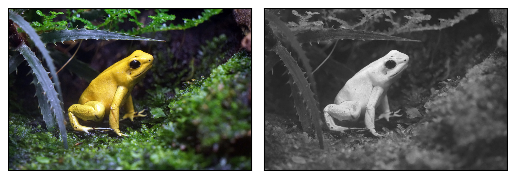
Example: Yellow = Red + Green.
Example: Detecting yellow
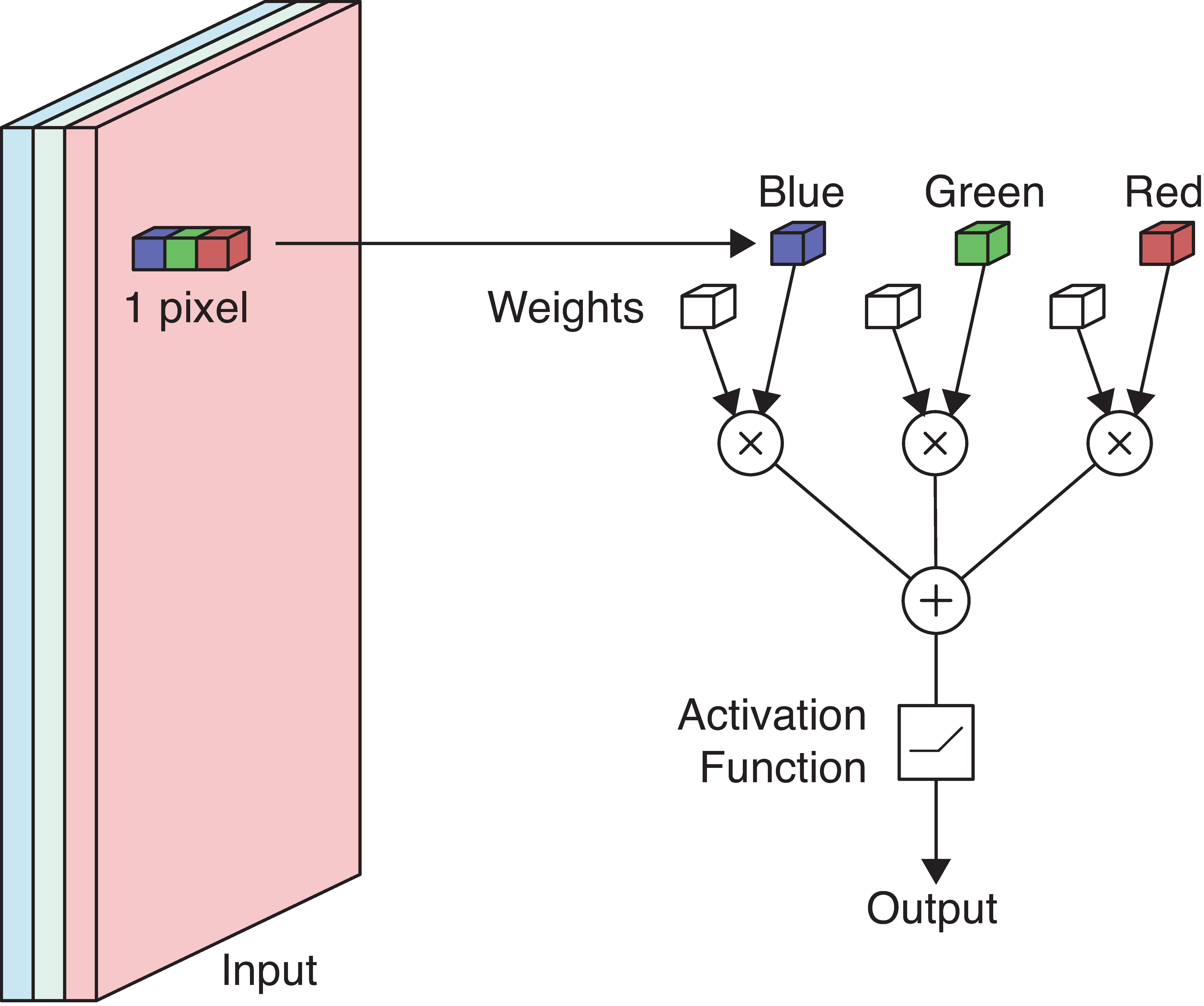
Apply a neuron to each pixel in the image.
If red/green \nearrow or blue \searrow then yellowness \nearrow.
Set RGB weights to 1, 1, -1.
Example: Detecting yellow II
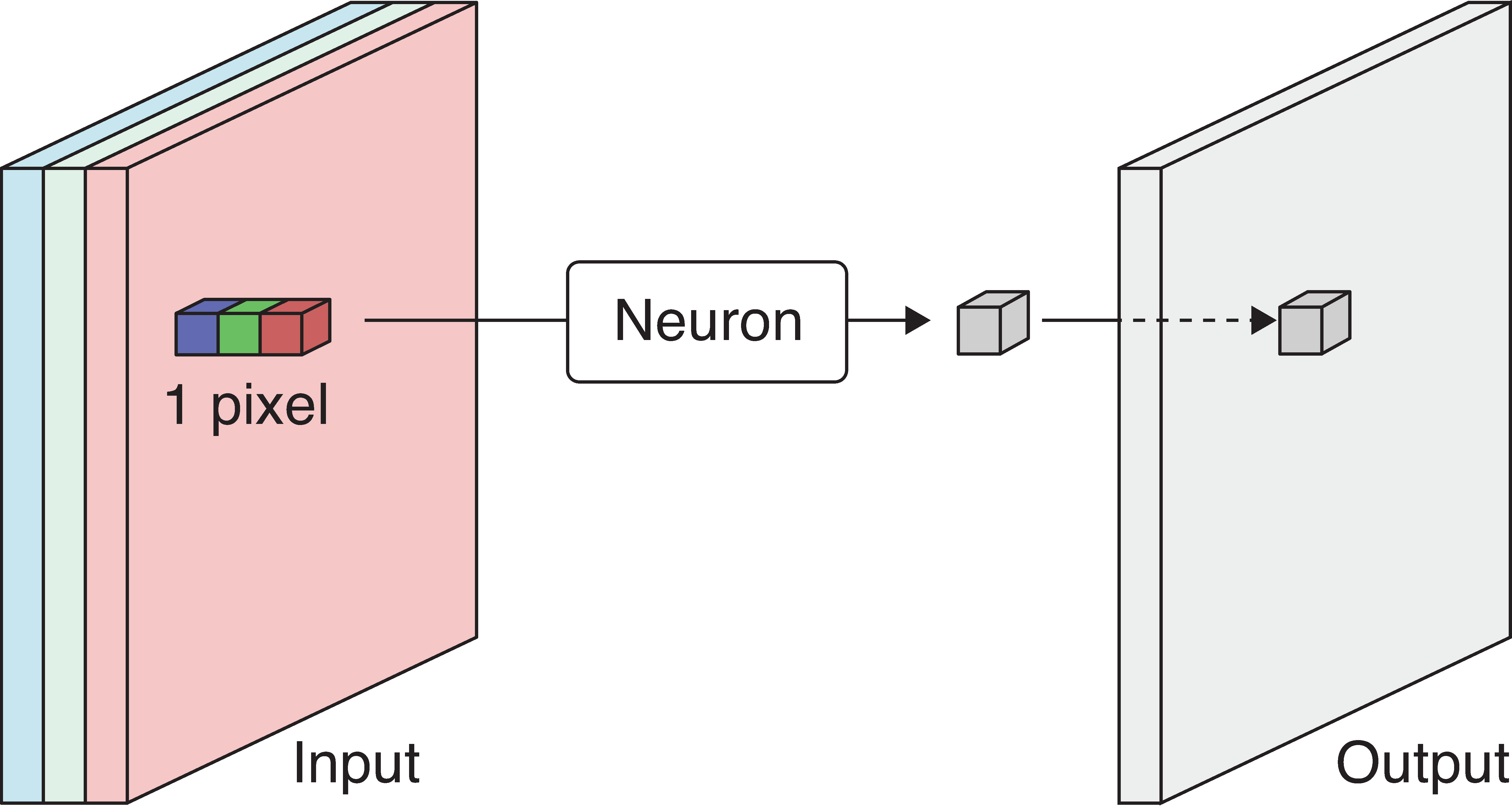
Scan the 3-channel input (colour image) with the neuron to produce a 1-channel output (grayscale image).
The output is produced by sweeping the neuron over the input. This is called convolution.
Example: Detecting yellow III
The more yellow the pixel in the colour image (left), the more white it is in the grayscale image.
The neuron or its weights is called a filter. We convolve the image with a filter, i.e. a convolutional filter.
Spatial filter
Example 3x3 filter
When a filter’s footprint is > 1 pixel, it is a spatial filter.
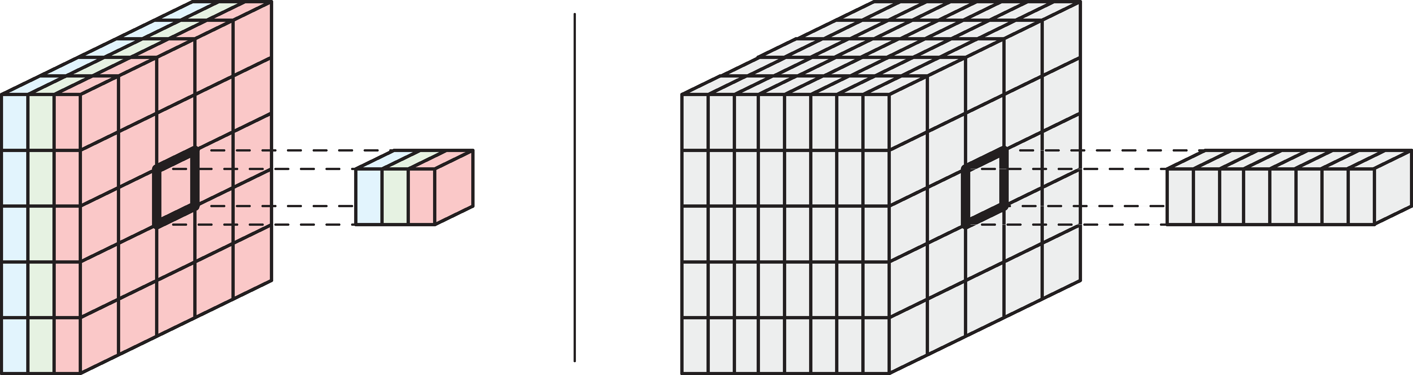
Multidimensional convolution
Need \# \text{ Channels in Input} = \# \text{ Channels in Filter}.
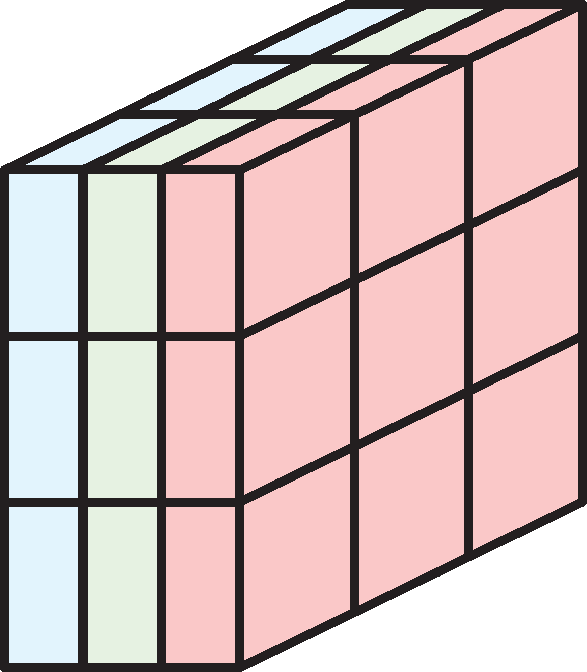
Example: a 3x3 filter with 3 channels, containing 27 weights.
Example: 3x3 filter over RGB input
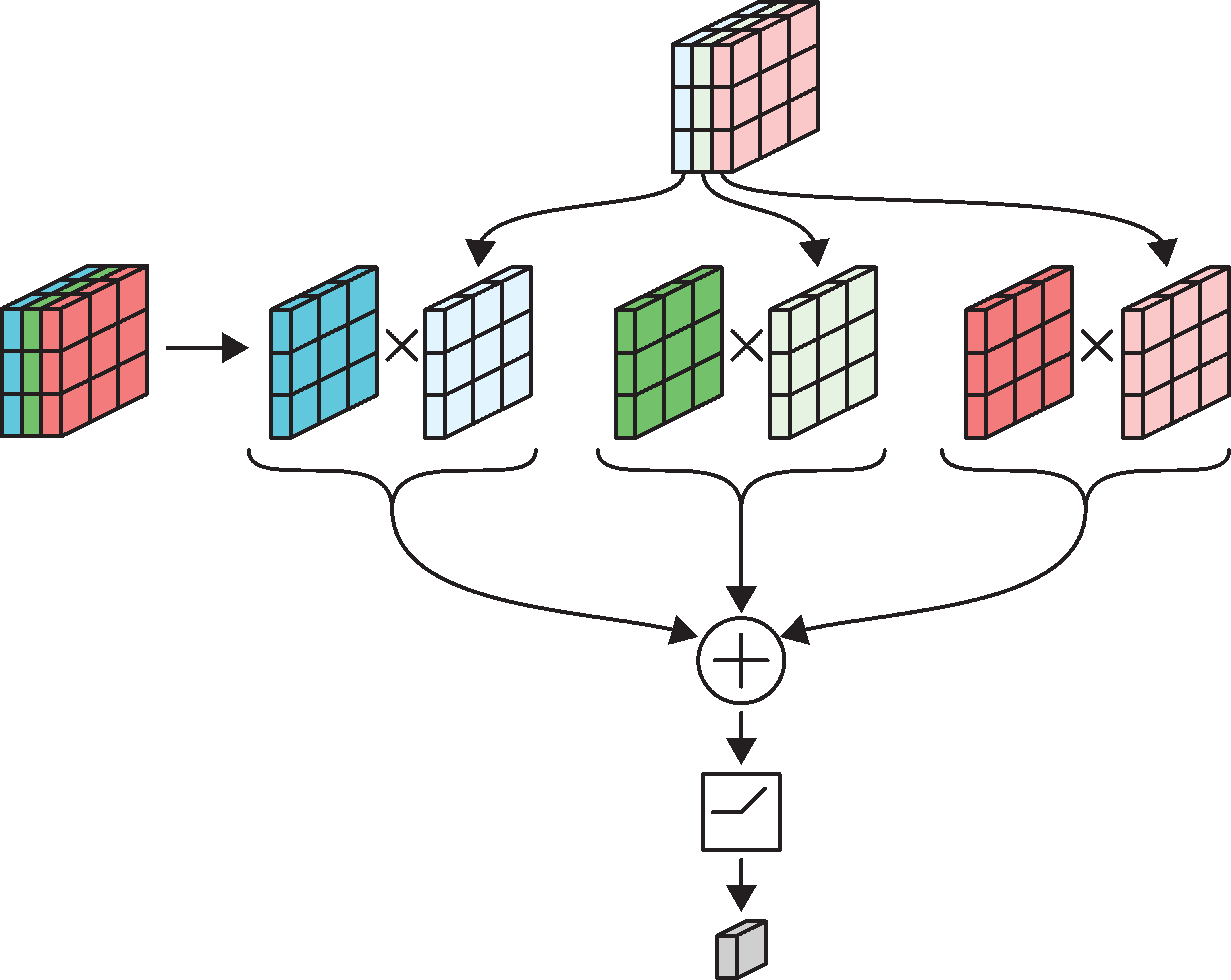
Each channel is multiplied separately & then added together.
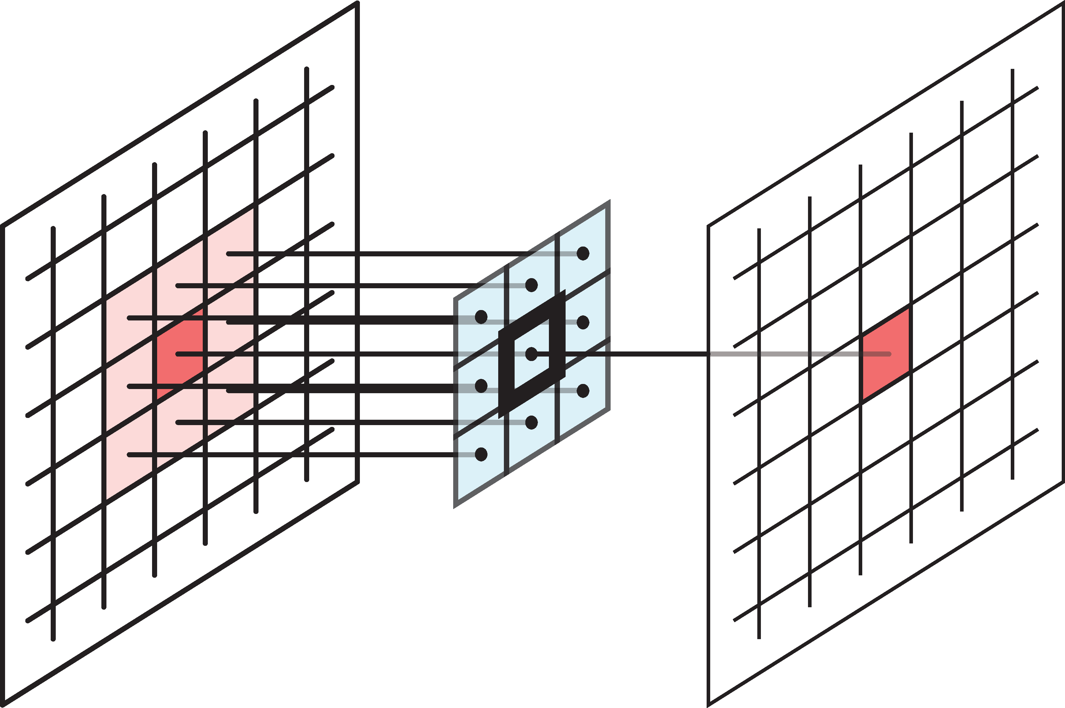
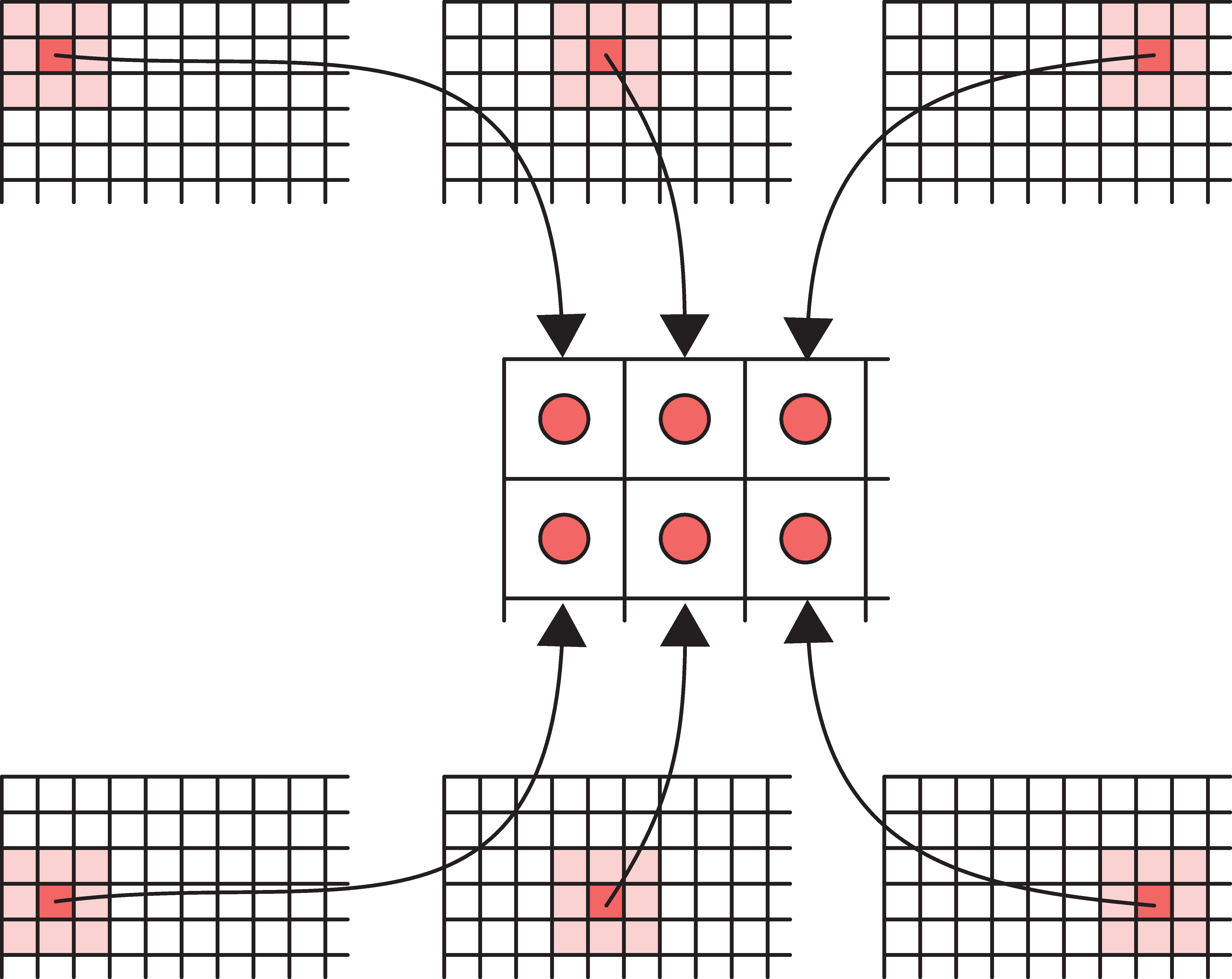
Input-output relationship
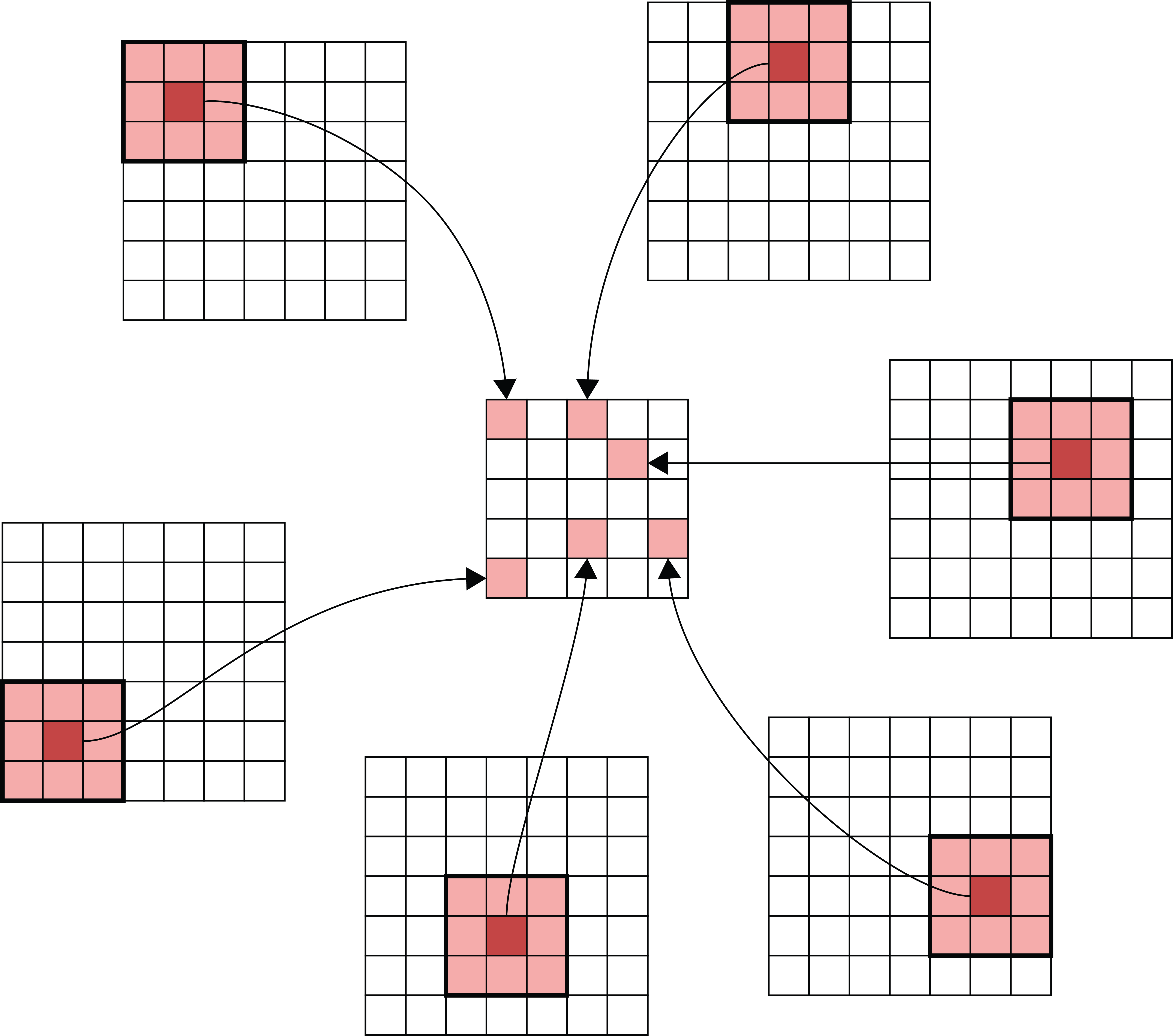
Matching the original image footprints against the output location.
Padding
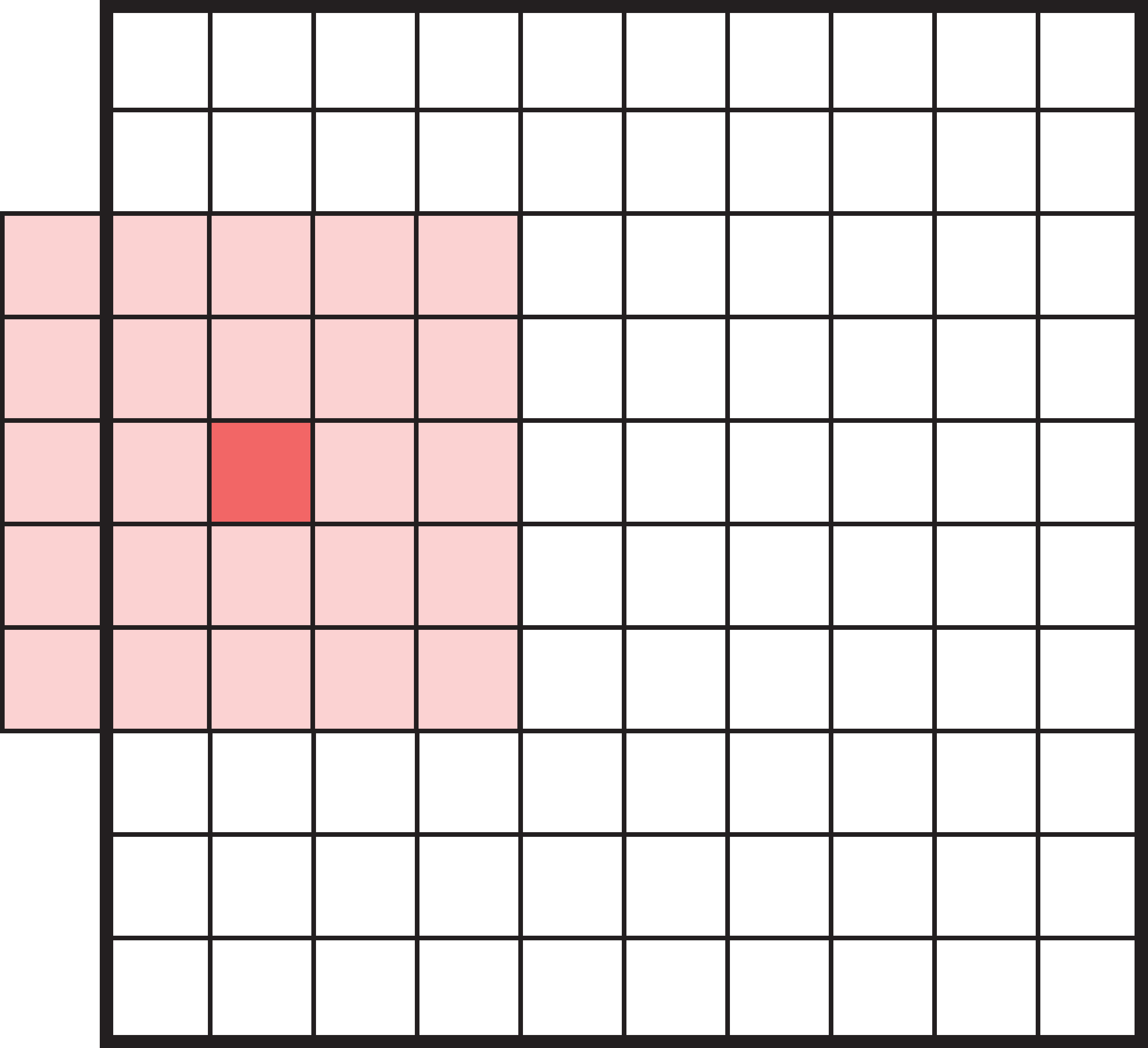
What happens when filters go off the edge of the input?
- How to avoid the filter’s receptive field falling off the side of the input.
- If we only scan the filter over places of the input where the filter can fit perfectly, it will lead to loss of information, especially after many filters.
Padding
Add a border of extra elements around the input, called padding. Normally we place zeros in all the new elements, called zero padding.
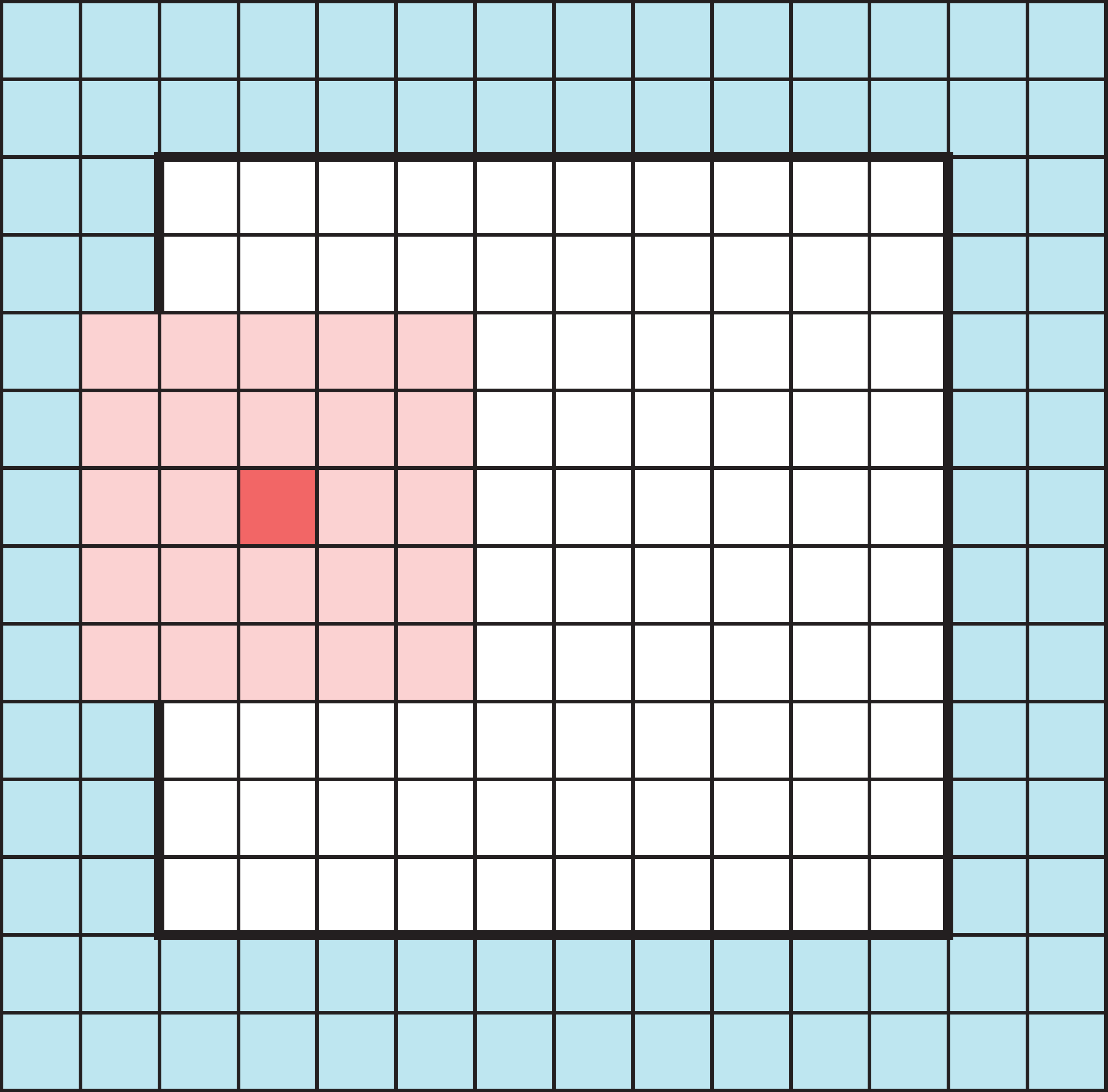
Padded values can be added to the outside of the input.
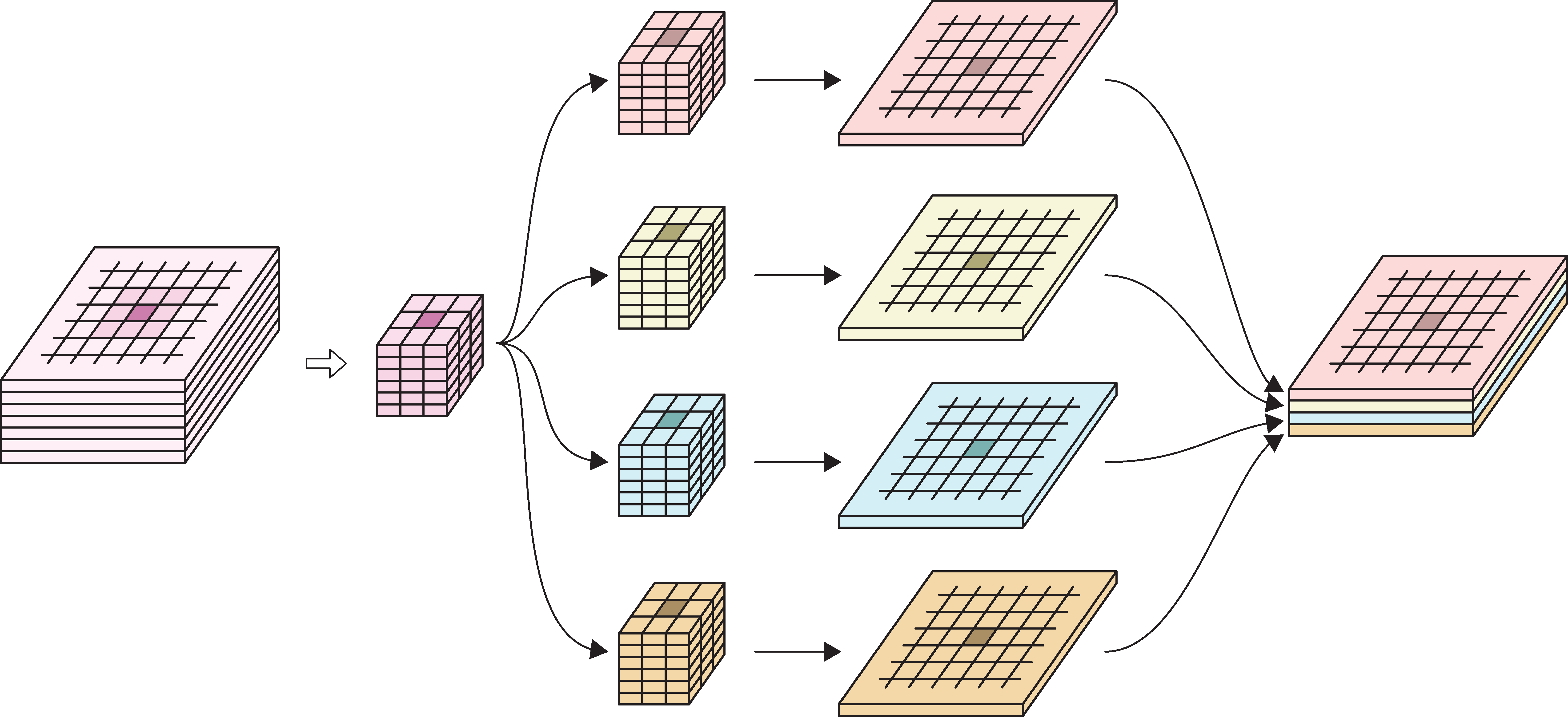
Example
In the image:
- 6-channel input tensor
- input pixels
- four 3x3 filters
- four output tensors
- final output tensor.
Example of 1x1 convolution
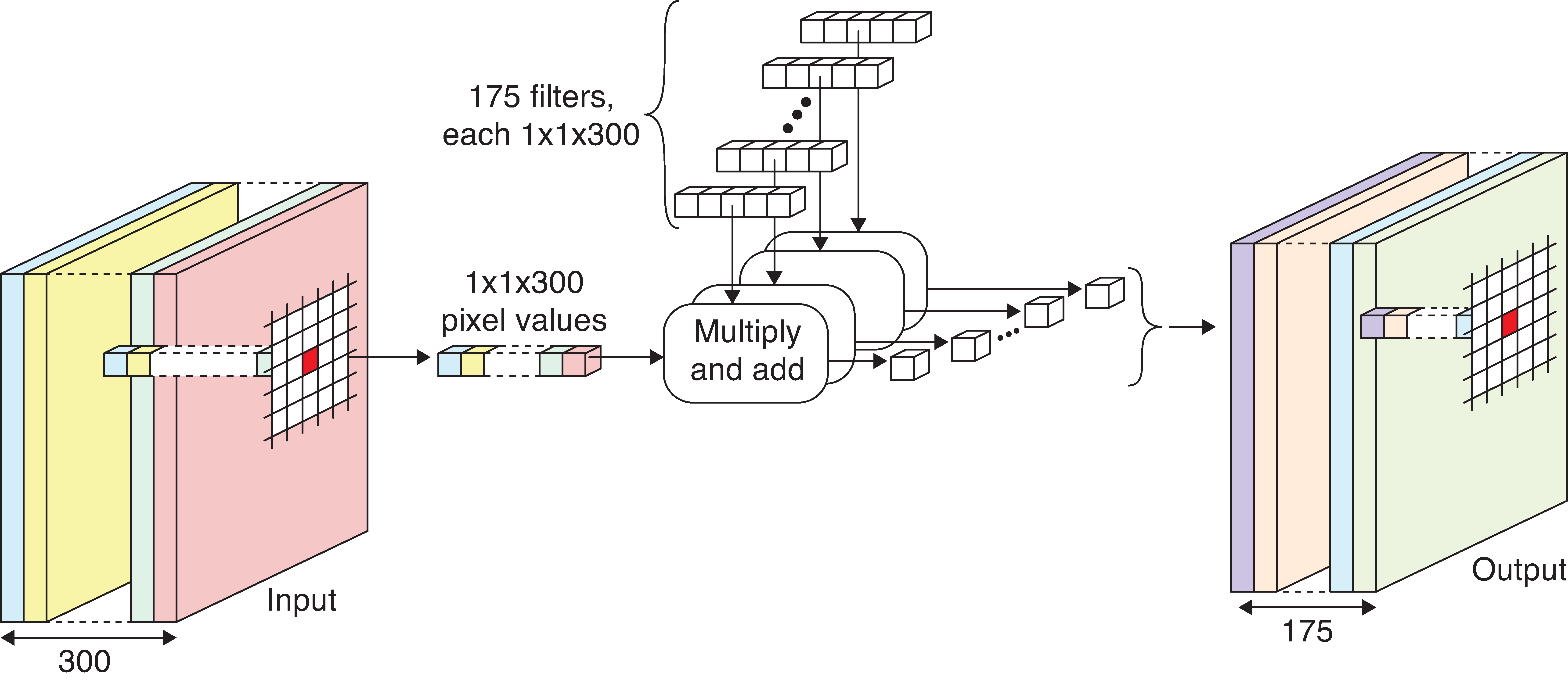
Example network with 1x1 convolution.
- Input tensor contains 300 channels.
- Use 175 1x1 filters in the convolution layer (300 weights each).
- Each filter produces a 1-channel output.
- Final output tensor has 175 channels.
Striding
We don’t have to go one pixel across/down at a time.
Example: Use a stride of three horizontally and two vertically.
Dimension of output will be smaller than input.
Choosing strides
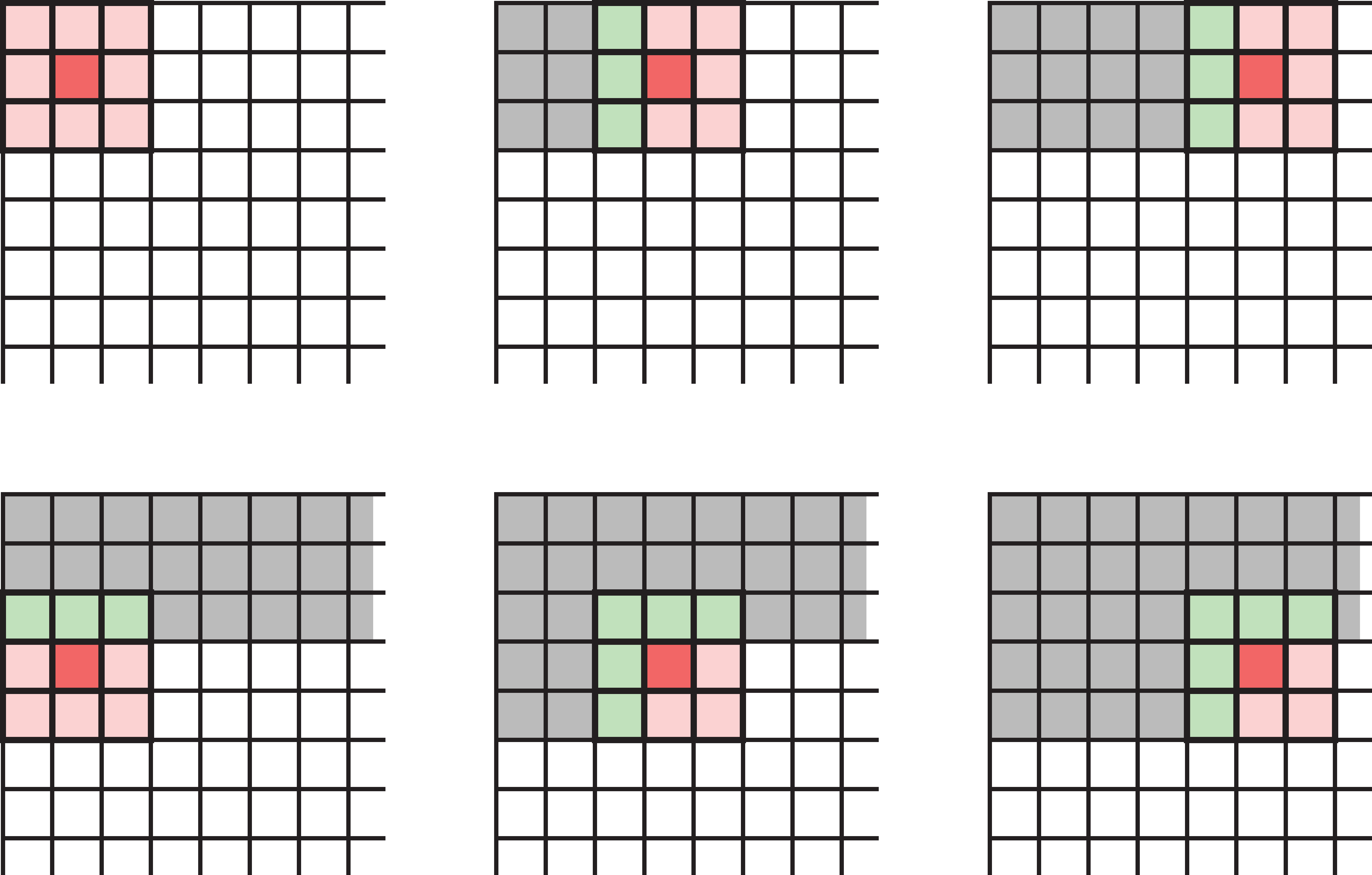
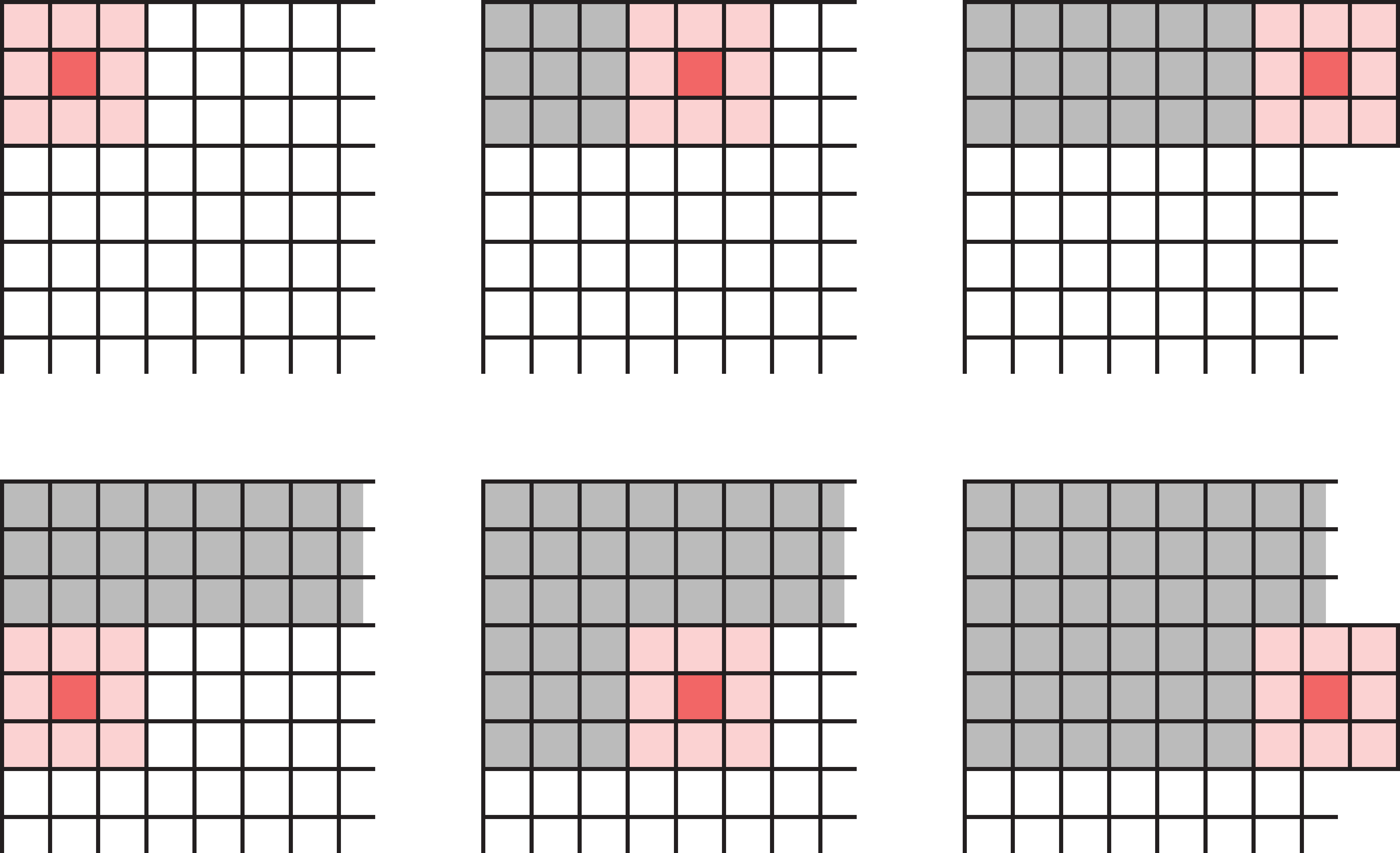
When a filter scans the input step by step, it processes the same input elements multiple times. Even with larger strides, this can still happen (left image).
If we want to save time, we can choose strides that prevents input elements from being used more than once. Example (right image): 3x3 filter, stride 3 in both directions.
Definition of CNN
A neural network that uses convolution layers is called a convolutional neural network.
Architecture
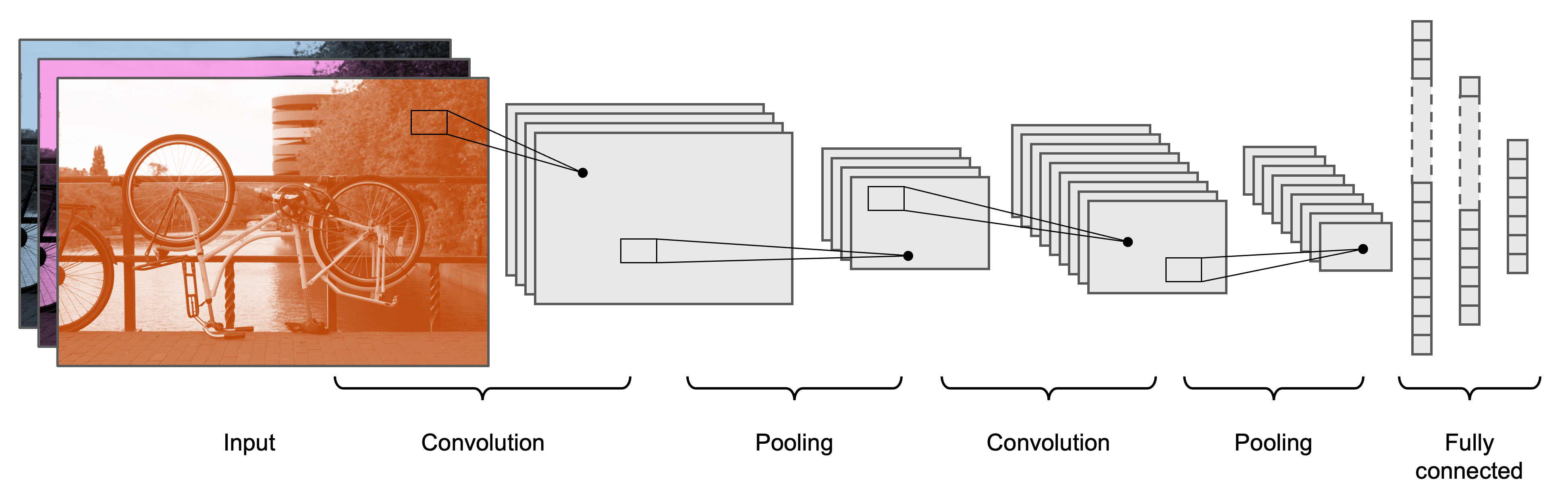
Typical CNN architecture.
Architecture II

Pooling
Pooling, or downsampling, is a technique to blur a tensor.
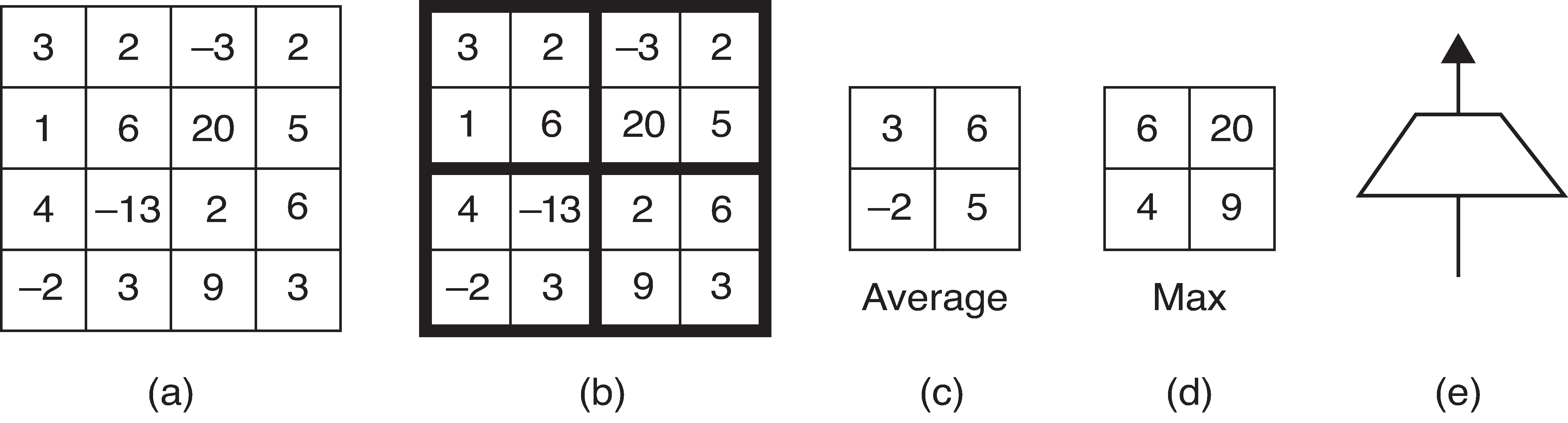
Illustration of pool operations.
(a): Input tensor (b): Subdivide input tensor into 2x2 blocks (c): Average pooling (d): Max pooling (e): Icon for a pooling layer
Pooling for multiple channels
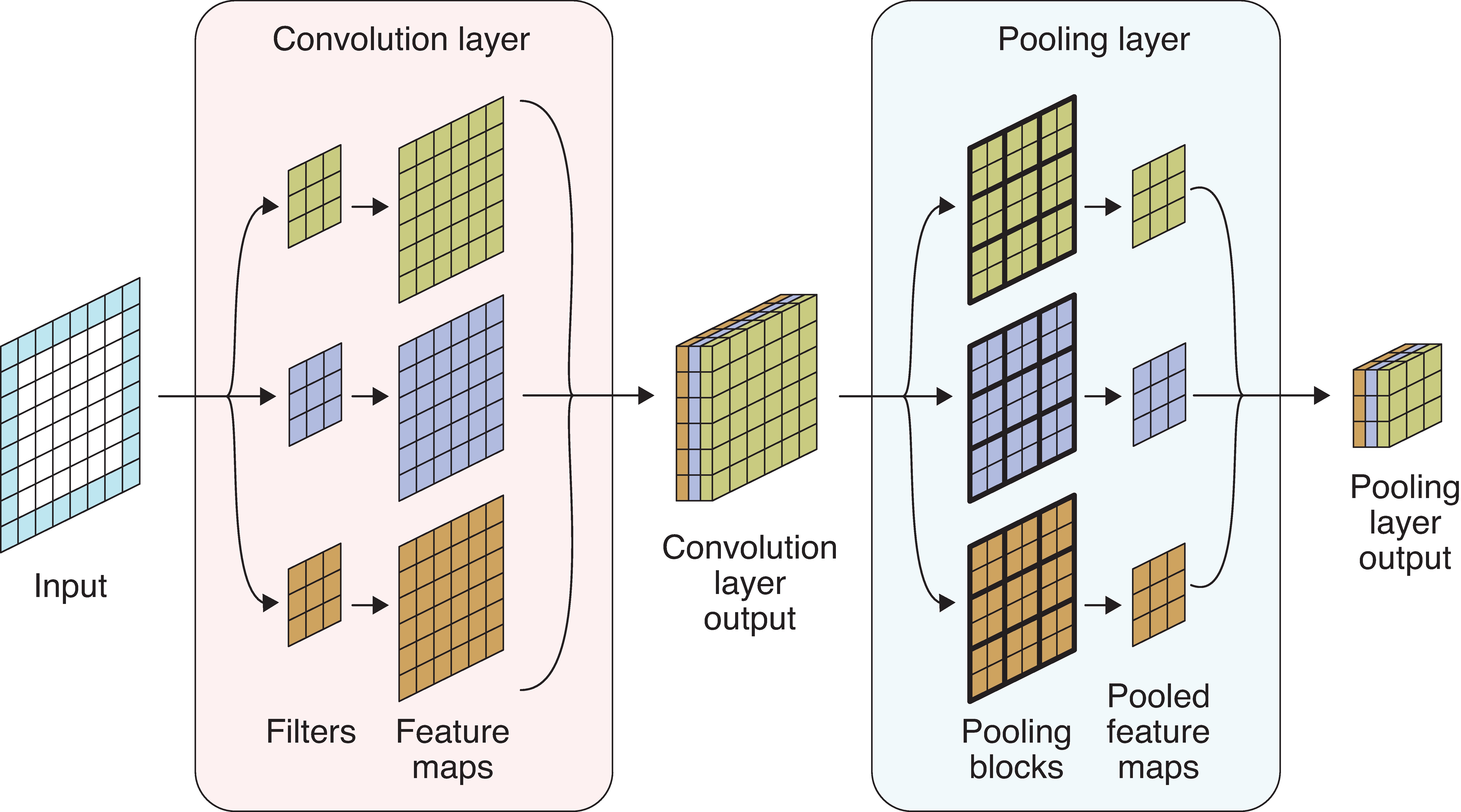
Pooling a multichannel input.
- Input tensor: 6x6 with 1 channel, zero padding.
- Convolution layer: Three 3x3 filters.
- Convolution layer output: 6x6 with 3 channels.
- Pooling layer: apply max pooling to each channel.
- Pooling layer output: 3x3, 3 channels.
Why/why not use pooling?
Why? Pooling reduces the size of tensors, therefore reduces memory usage and execution time (recall that 1x1 convolution reduces the number of channels in a tensor).
Why not?
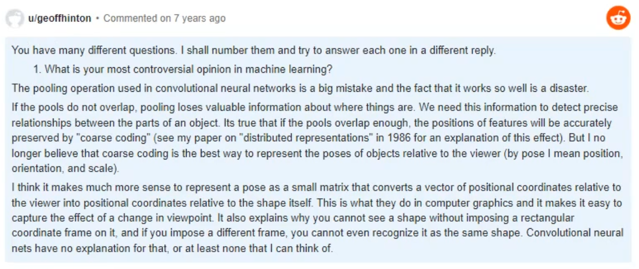
Geoffrey Hinton
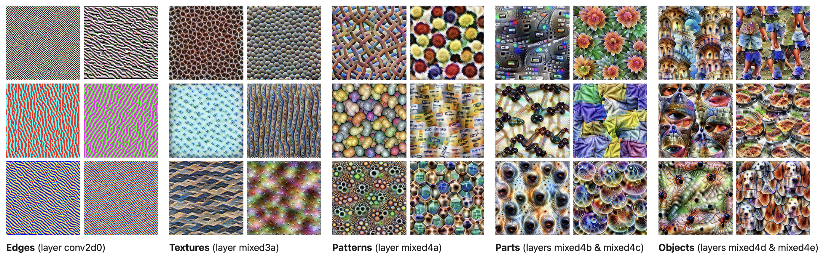
What do the CNN layers learn?
MNIST Dataset
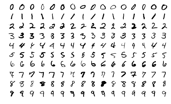
The MNIST dataset.
CASIA Chinese handwriting database
Dataset source: Institute of Automation of Chinese Academy of Sciences (CASIA)
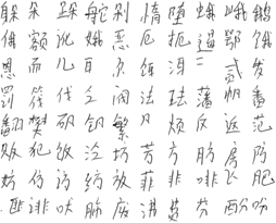
A 13 GB dataset of 3,999,571 handwritten characters.
Number of images for each character
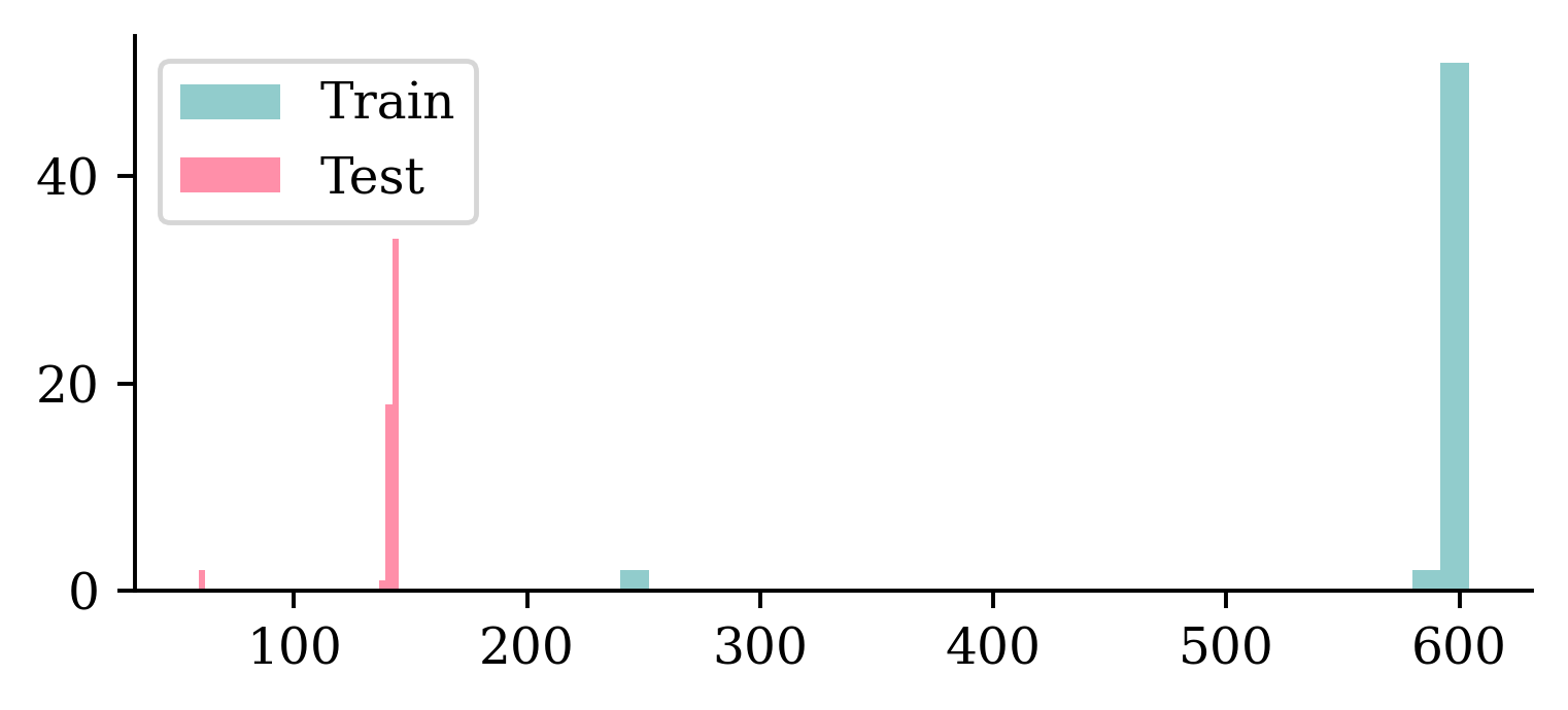
It differs, but basically ~600 training and ~140 test images per character. A couple of characters have a lot less of both though.
Checking the dimensions II
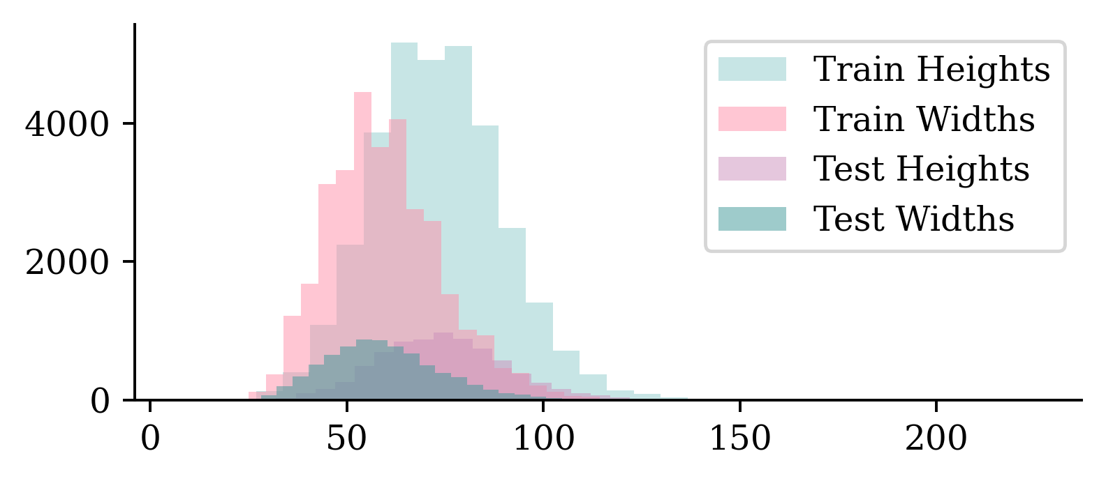
The images are taller than they are wide. We have more training images than test images.
Checking the dimensions III
plt.hist(train_heights, bins=30, alpha=0.5, label="Train Heights", density=True)
plt.hist(train_widths, bins=30, alpha=0.5, label="Train Widths", density=True)
plt.hist(test_heights, bins=30, alpha=0.5, label="Test Heights", density=True)
plt.hist(test_widths, bins=30, alpha=0.5, label="Test Widths", density=True)
plt.legend();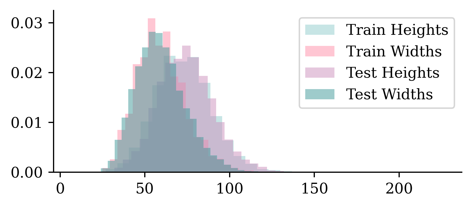
Checking the dimensions IV
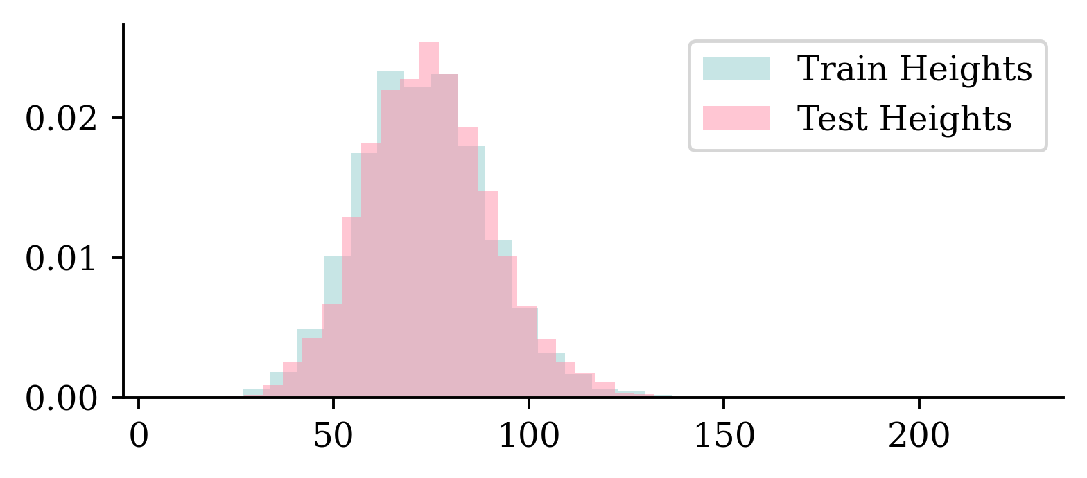
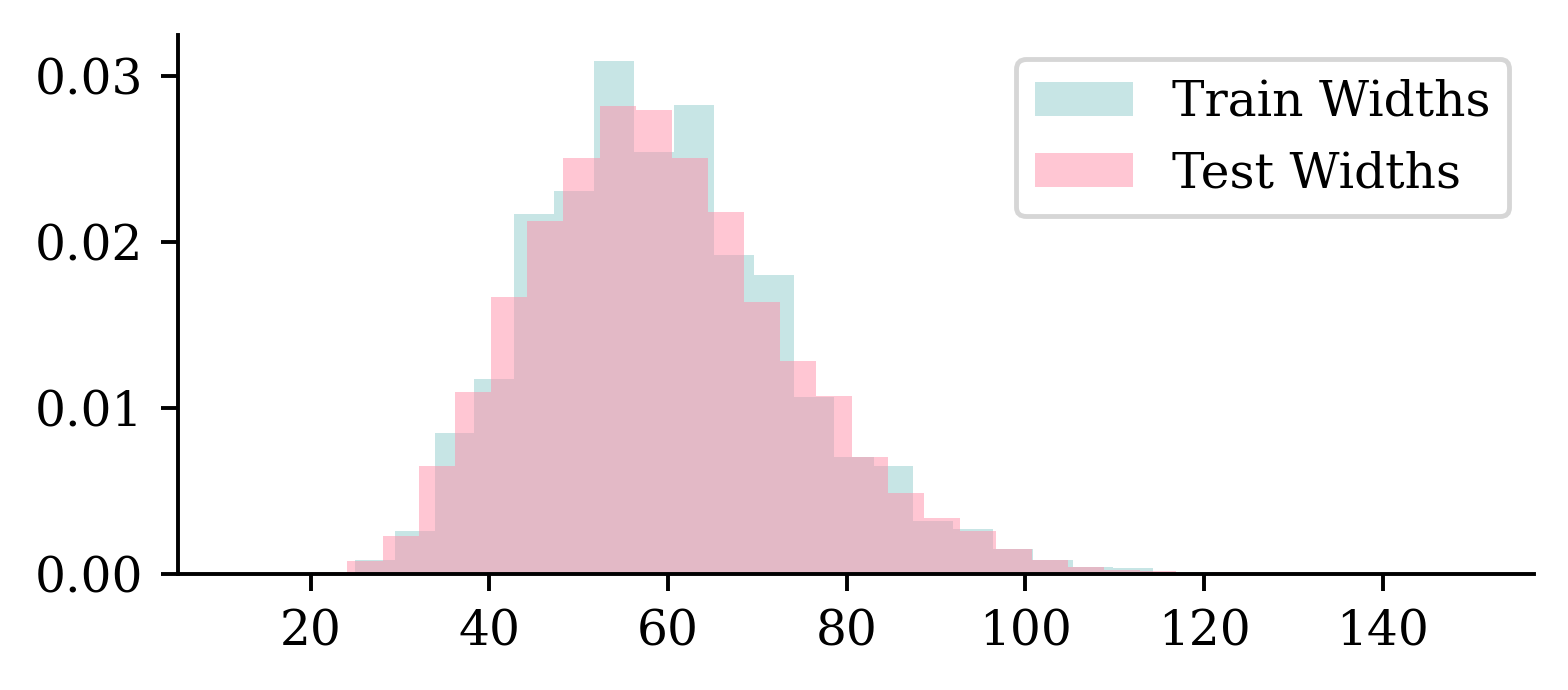
The distribution of dimensions are pretty similar between training and test sets.
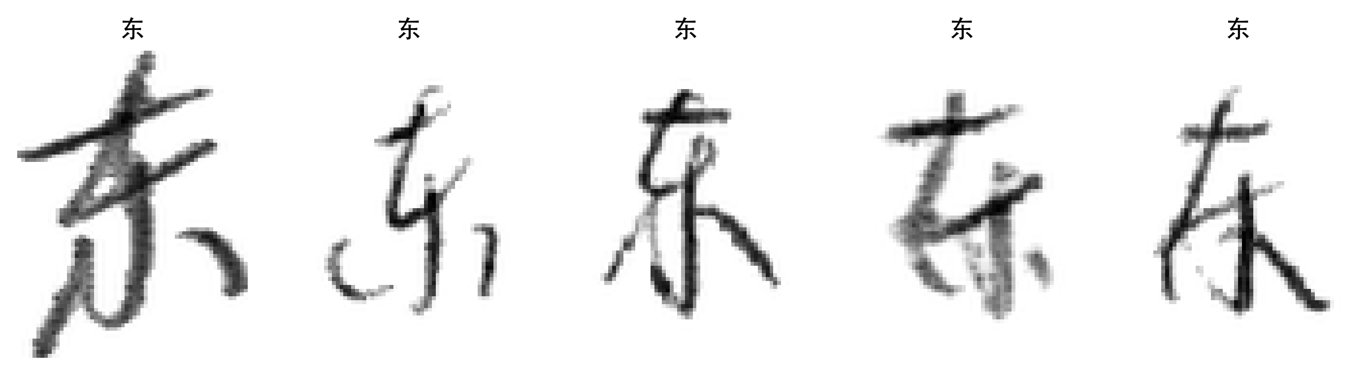
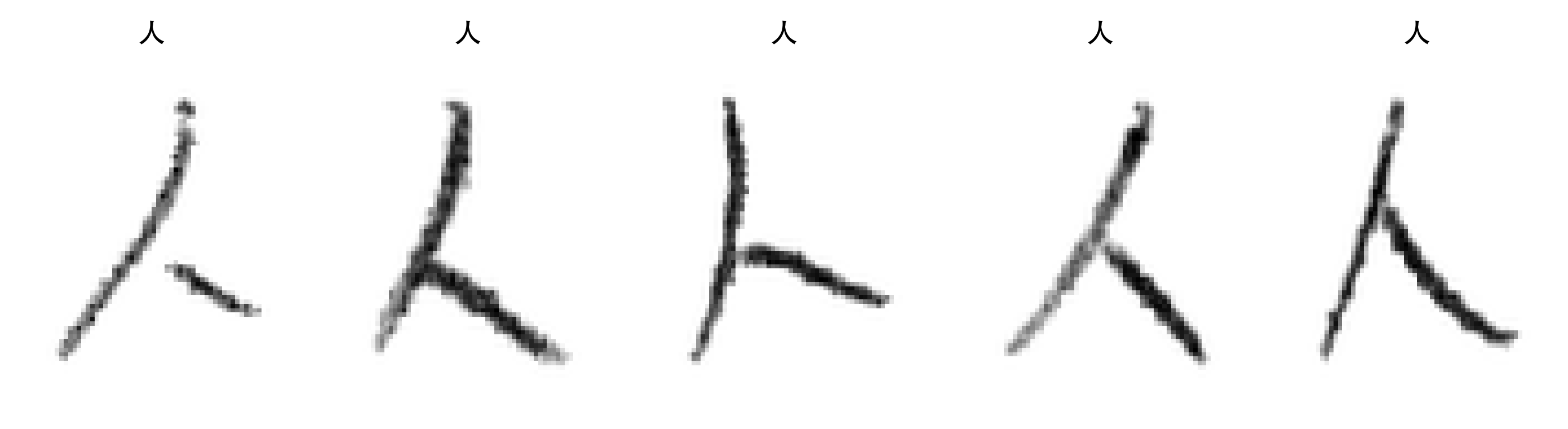
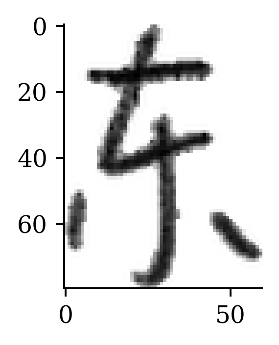
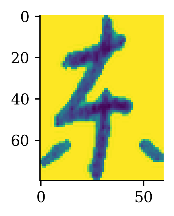
Plotting some training characters
Without the colourmap..
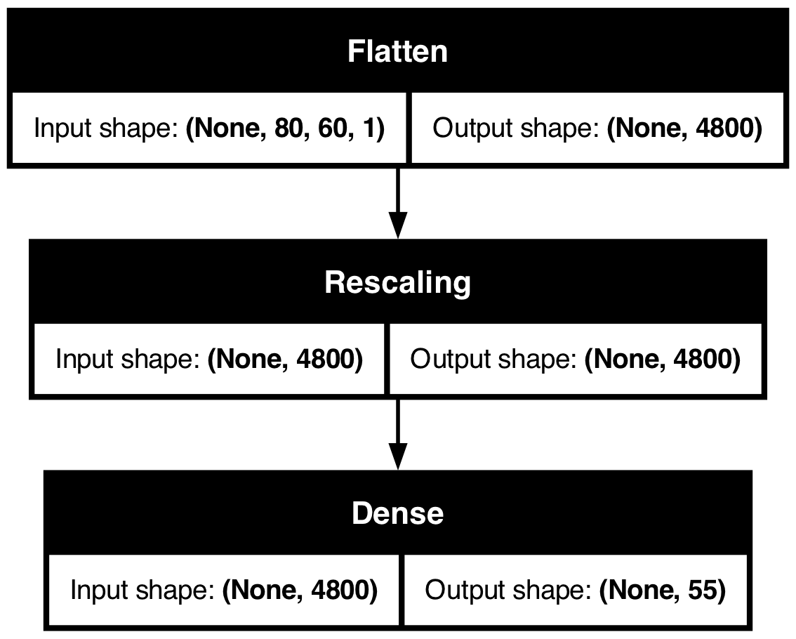
Make a logistic regression
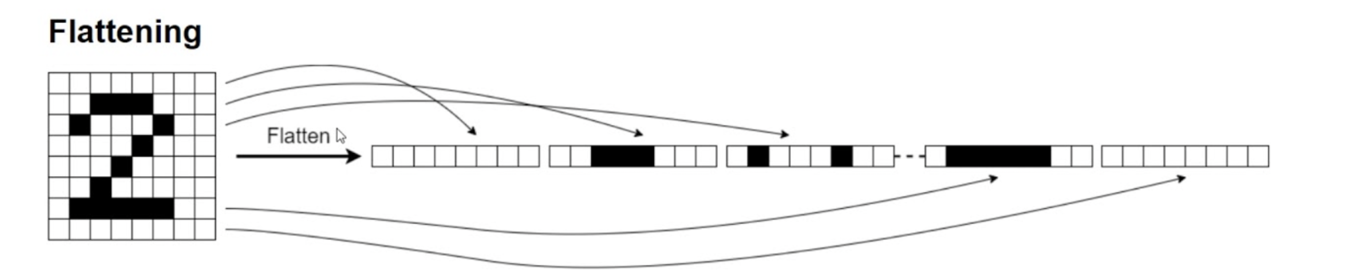
Basically pretend it’s not an image
Tip
The Rescaling layer will rescale the intensities to [0, 1].
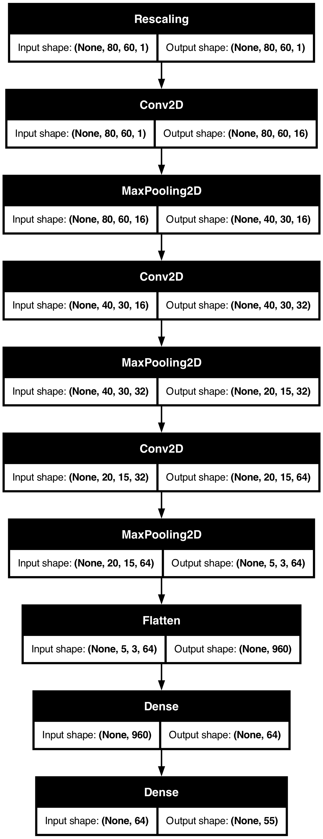
Plot the model
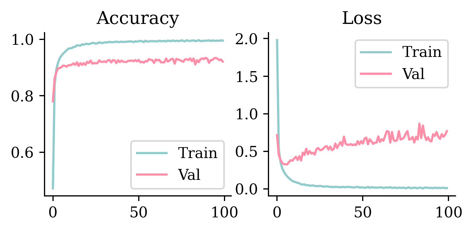
Plot the loss/accuracy curves
Code
def plot_history(history):
    epochs = range(len(history["loss"]))

    plt.subplot(1, 2, 1)
    plt.plot(epochs, history["accuracy"], label="Train")
    plt.plot(epochs, history["val_accuracy"], label="Val")
    plt.legend(loc="lower right")
    plt.title("Accuracy")

    plt.subplot(1, 2, 2)
    plt.plot(epochs, history["loss"], label="Train")
    plt.plot(epochs, history["val_loss"], label="Val")
    plt.legend(loc="upper right")
    plt.title("Loss")
    plt.show()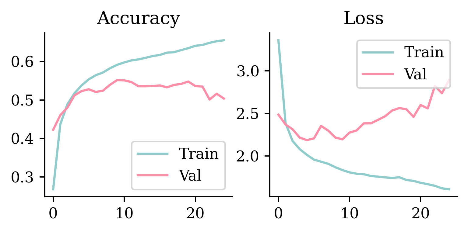
Plot the CNN
Plot the loss/accuracy curves
Predict on the test set II

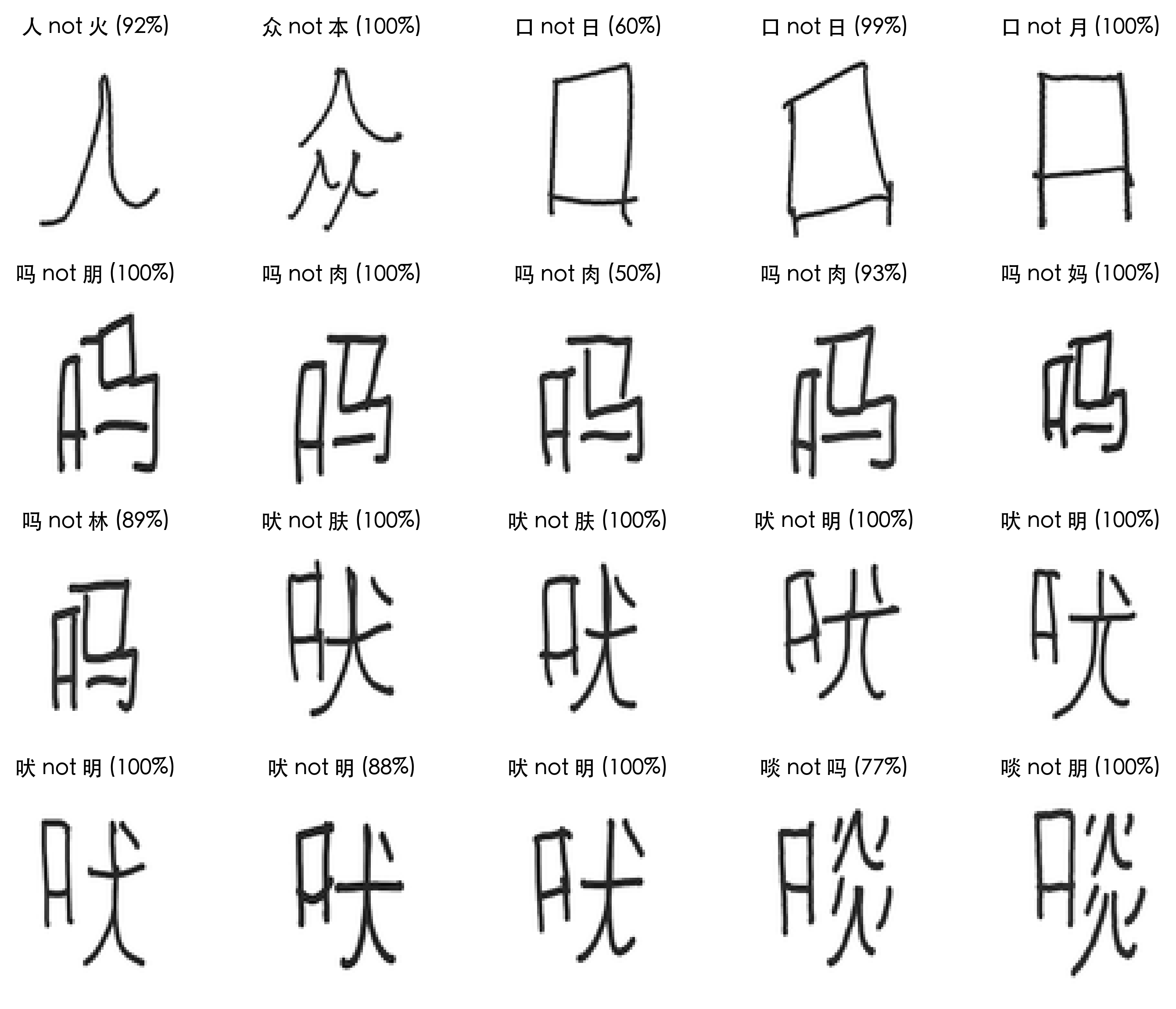
Take a look at the failure cases
Code
def plot_failed_predictions(X, y, class_names, max_errors = 20,
            num_rows = 4, num_cols = 5, title_font=CHINESE_FONT):
    plt.figure(figsize=(num_cols * 2, num_rows * 2))
    errors = 0
    y_pred = model.predict(X, verbose=0)
    y_pred_classes = y_pred.argmax(axis=1)
    y_pred_probs = keras.ops.convert_to_numpy(keras.ops.softmax(y_pred)).max(axis=1)
    for i in range(len(y_pred)):
        if errors >= max_errors:
            break
        if y_pred_classes[i] != y[i]:
            plt.subplot(num_rows, num_cols, errors + 1)
            plt.imshow(X[i], cmap="gray")
            true_class = class_names[y[i]]
            pred_class = class_names[y_pred_classes[i]]
            conf = y_pred_probs[i]
            msg = f"{true_class} not {pred_class} ({conf*100:.0f}%)"
            plt.title(msg, fontproperties=title_font)
            plt.axis("off")
            errors += 1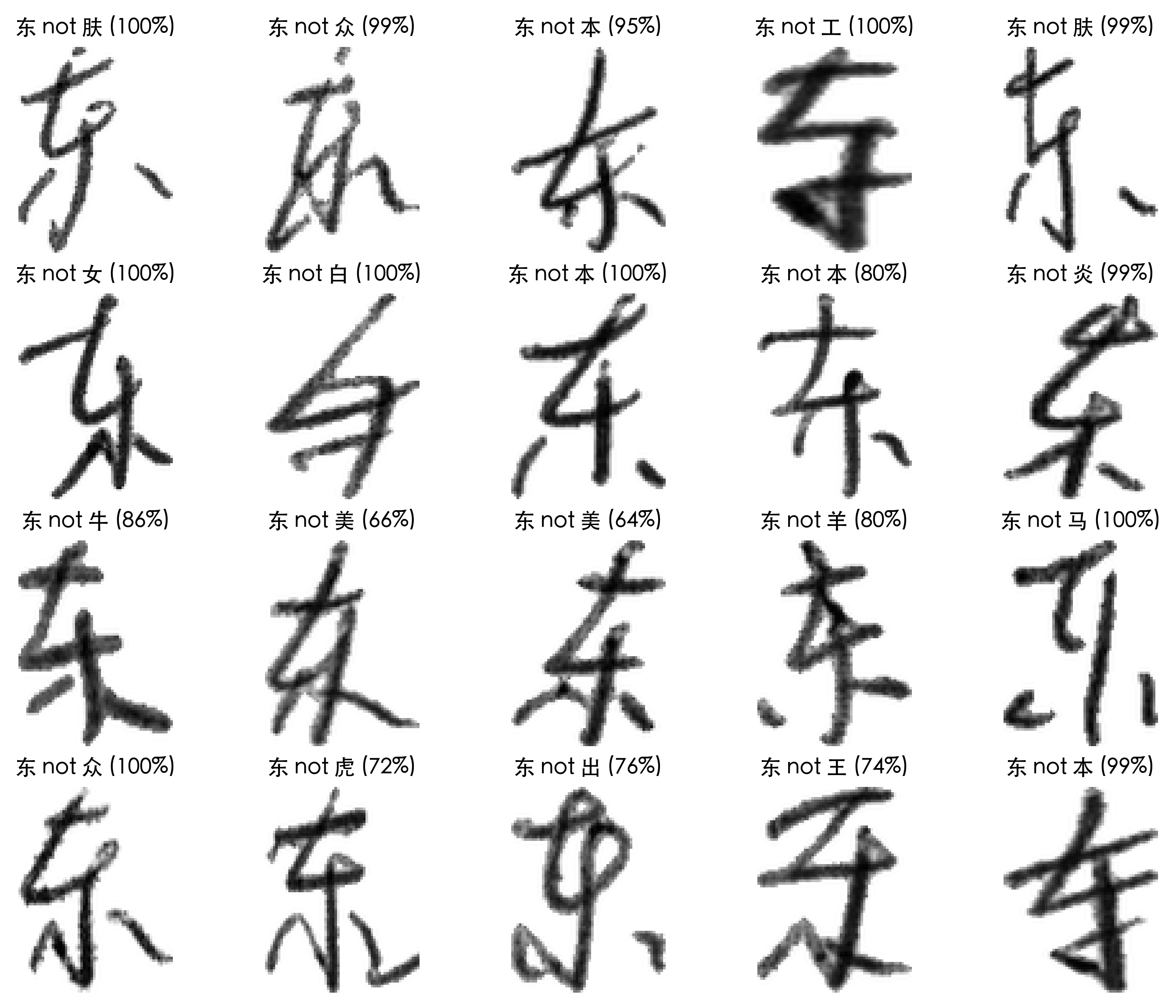
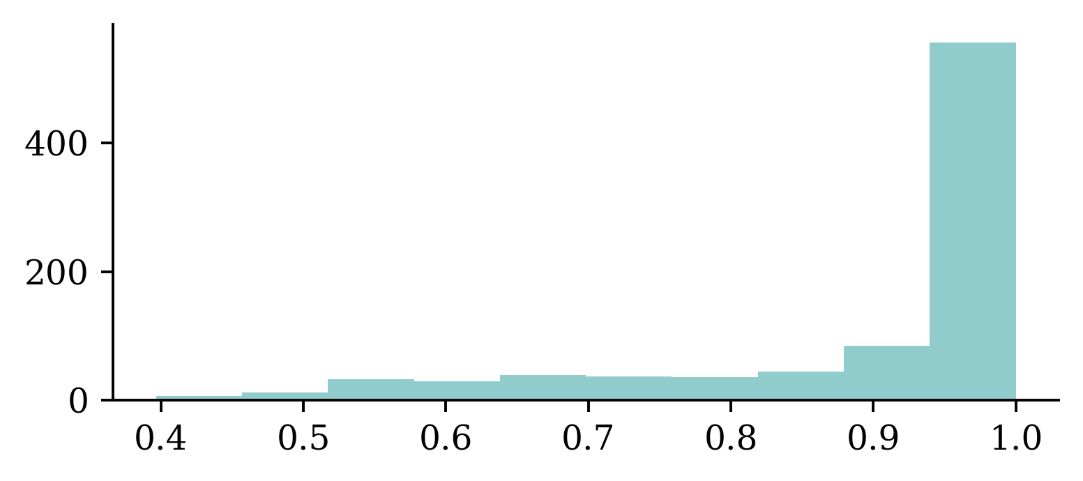
Confidence of predictions
y_log = model.predict(X_test, verbose=0)
y_pred = keras.ops.convert_to_numpy(keras.activations.softmax(y_log))
y_pred_class = np.argmax(y_pred, axis=1)
y_pred_prob = y_pred[np.arange(y_pred.shape[0]), y_pred_class]

confidence_when_correct = y_pred_prob[y_pred_class == y_test]
confidence_when_wrong = y_pred_prob[y_pred_class != y_test]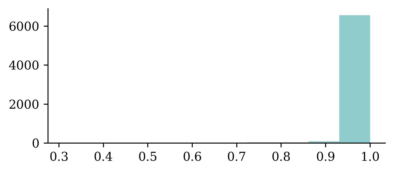
Another test set
55 poorly written Mandarin characters (55 \times 7 = 385).
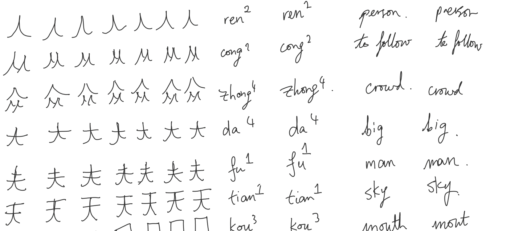
Dataset of notes when learning/practising basic characters.
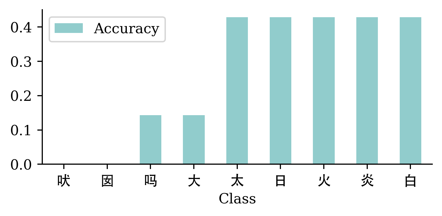
Errors
Least (AI-) legible characters
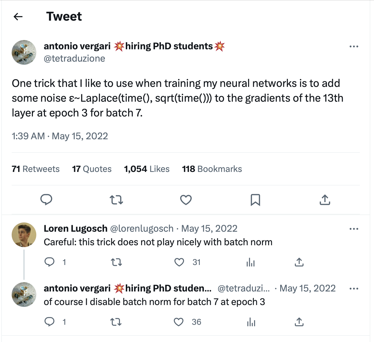
Trial & error
Frankly, a lot of this is just ‘enlightened’ trial and error.
Demo: Object classification

Data Augmentation
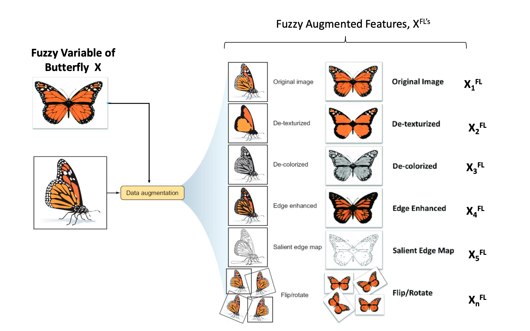
Examples of data augmentation.
Inception module (2013)
Used in ILSVRC 2013 winning solution (top-5 error < 7%).
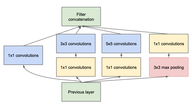

VGGNet was the runner-up.
GoogLeNet / Inception_v0 (2014)
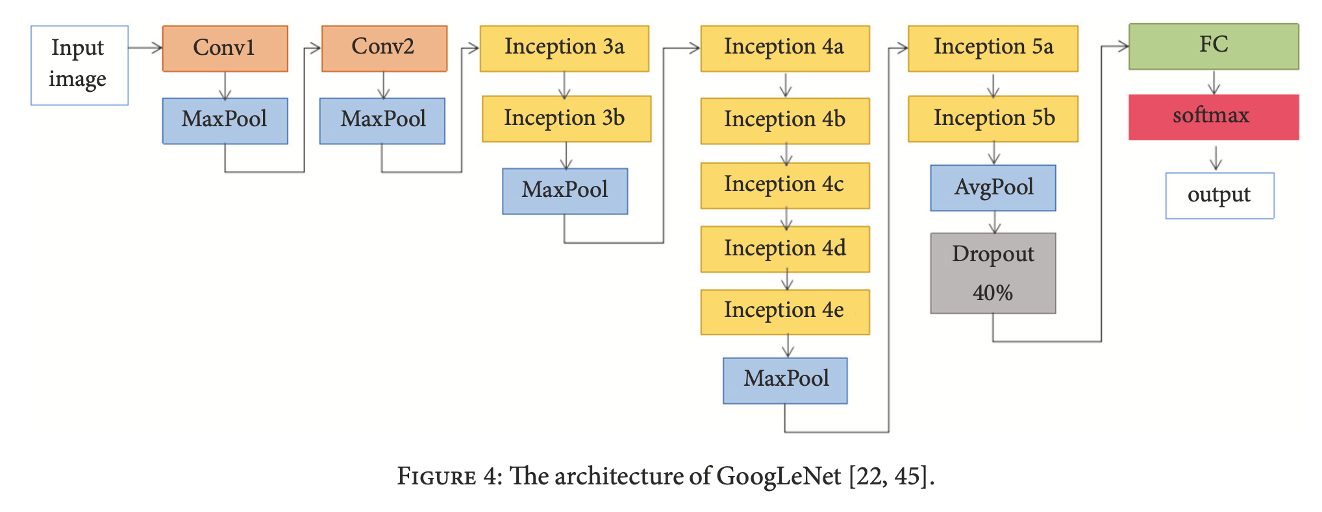
Schematic of the GoogLeNet architecture.
Depth is important for image tasks
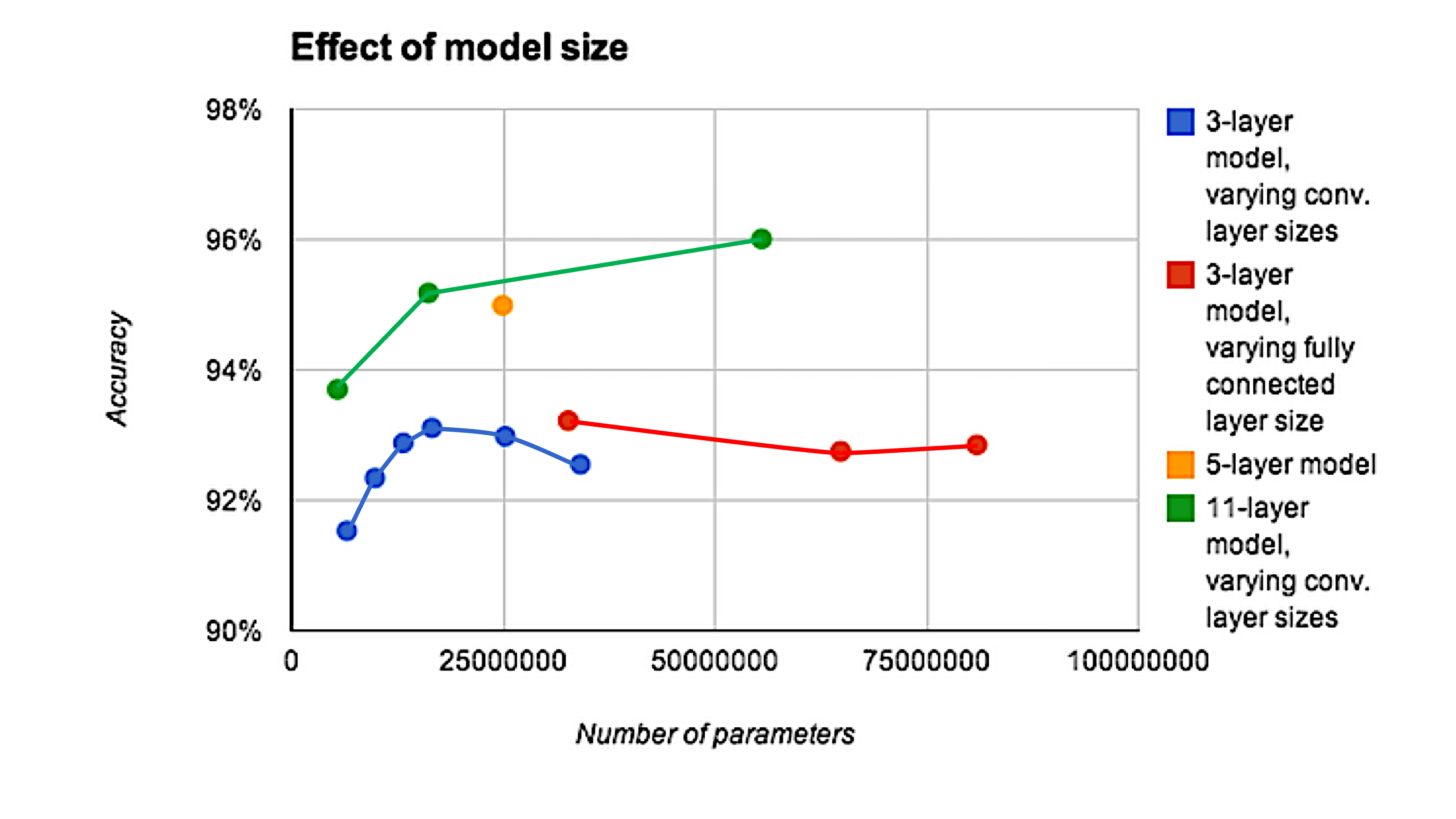
Deeper models aren’t just better because they have more parameters.
Residual connection
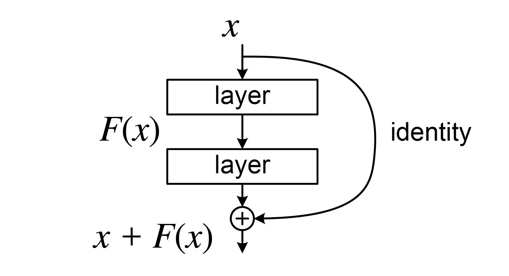
Illustration of a residual connection.
Predicted classes (MobileNet)
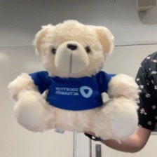
Image #0:
n04399382 - teddy 89%
n04254120 - soap_dispenser 7%
n04462240 - toyshop 2%
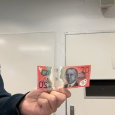
Image #1:
n03075370 - combination_lock 30%
n04019541 - puck 26%
n03666591 - lighter 10%
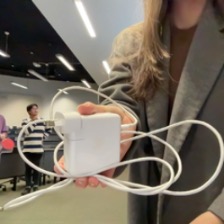
Image #2:
n04009552 - projector 20%
n03908714 - pencil_sharpener 17%
n02951585 - can_opener 9%

Predicted classes (MobileNetV2)
Image #0:
 n04399382 - teddy 44%
 n04462240 - toyshop 3%
 n03476684 - hair_slide 3%

Image #1:
 n03075370 - combination_lock 59%
 n03843555 - oil_filter 6%
 n04023962 - punching_bag 3%

Image #2:
 n03529860 - home_theater 11%
 n03041632 - cleaver 10%
 n04209133 - shower_cap 6%
Predicted classes (InceptionV3)
Image #0:
 n04399382 - teddy 87%
 n04162706 - seat_belt 2%
 n04462240 - toyshop 2%

Image #1:
 n04023962 - punching_bag 13%
 n03337140 - file 7%
 n02992529 - cellular_telephone 3%

Image #2:
 n04005630 - prison 4%
 n03337140 - file 4%
 n06596364 - comic_book 2%
Predicted classes II (MobileNet)
Image #0:
n03483316 - hand_blower 21%
n03271574 - electric_fan 8%
n07579787 - plate 4%
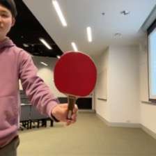
Image #1:
n03942813 - ping-pong_ball 88%
n02782093 - balloon 3%
n04023962 - punching_bag 1%
Image #2:
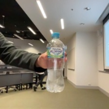
n04557648 - water_bottle 31%
n04336792 - stretcher 14%
n03868863 - oxygen_mask 7%
Predicted classes II (MobileNetV2)
Image #0:
 n03868863 - oxygen_mask 37%
 n03483316 - hand_blower 7%
 n03271574 - electric_fan 7%

Image #1:
 n03942813 - ping-pong_ball 29%
 n04270147 - spatula 12%
 n03970156 - plunger 8%

Image #2:
 n02815834 - beaker 40%
 n03868863 - oxygen_mask 16%
 n04557648 - water_bottle 4%
Predicted classes II (InceptionV3)
Image #0:
 n02815834 - beaker 19%
 n03179701 - desk 15%
 n03868863 - oxygen_mask 9%

Image #1:
 n03942813 - ping-pong_ball 87%
 n02782093 - balloon 8%
 n02790996 - barbell 0%

Image #2:
 n04557648 - water_bottle 55%
 n03983396 - pop_bottle 9%
 n03868863 - oxygen_mask 7%
Predicted classes III (MobileNet)
Image #0:
 n04350905 - suit 39%
 n04591157 - Windsor_tie 34%
 n02749479 - assault_rifle 13%

Image #1:
 n03529860 - home_theater 25%
 n02749479 - assault_rifle 9%
 n04009552 - projector 5%

Image #2:
 n03529860 - home_theater 9%
 n03924679 - photocopier 7%
 n02786058 - Band_Aid 6%


Predicted classes III (MobileNetV2)
Image #0:
 n04350905 - suit 34%
 n04591157 - Windsor_tie 8%
 n03630383 - lab_coat 7%

Image #1:
 n04023962 - punching_bag 9%
 n04336792 - stretcher 4%
 n03529860 - home_theater 4%

Image #2:
 n04404412 - television 42%
 n02977058 - cash_machine 6%
 n04152593 - screen 3%
Predicted classes III (InceptionV3)
Image #0:
n04350905 - suit 25%
n04591157 - Windsor_tie 11%
n03630383 - lab_coat 6%
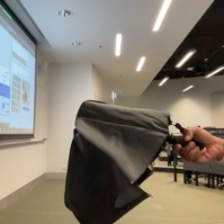
Image #1:
n04507155 - umbrella 52%
n04404412 - television 2%
n03529860 - home_theater 2%
Image #2:
n04404412 - television 17%
n02777292 - balance_beam 7%
n03942813 - ping-pong_ball 6%
The original pretrained model
