import random
from pathlib import Path

import matplotlib.pyplot as plt
import matplotlib.font_manager as fm
from matplotlib.image import imread
from matplotlib.pyplot import imshow
import numpy as np
import pandas as pd
from PIL import Image

import keras
from keras.models import Sequential, Model
from keras.layers import (Dense, Input, Rescaling, Flatten,
    Conv2D, MaxPooling2D, GlobalAveragePooling2D)
from keras.callbacks import EarlyStopping
from keras.utils import plot_model

from sklearn.model_selection import train_test_split
from sklearn.preprocessing import StandardScaler

from directory_tree import DisplayTree
import optunaComputer Vision
ACTL3143 & ACTL5111 Deep Learning for Actuaries
Facial analytics and life insurance

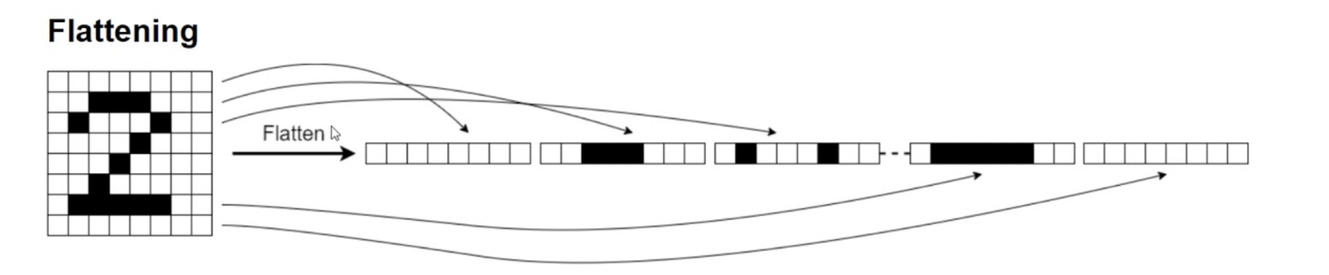
Shapes of data
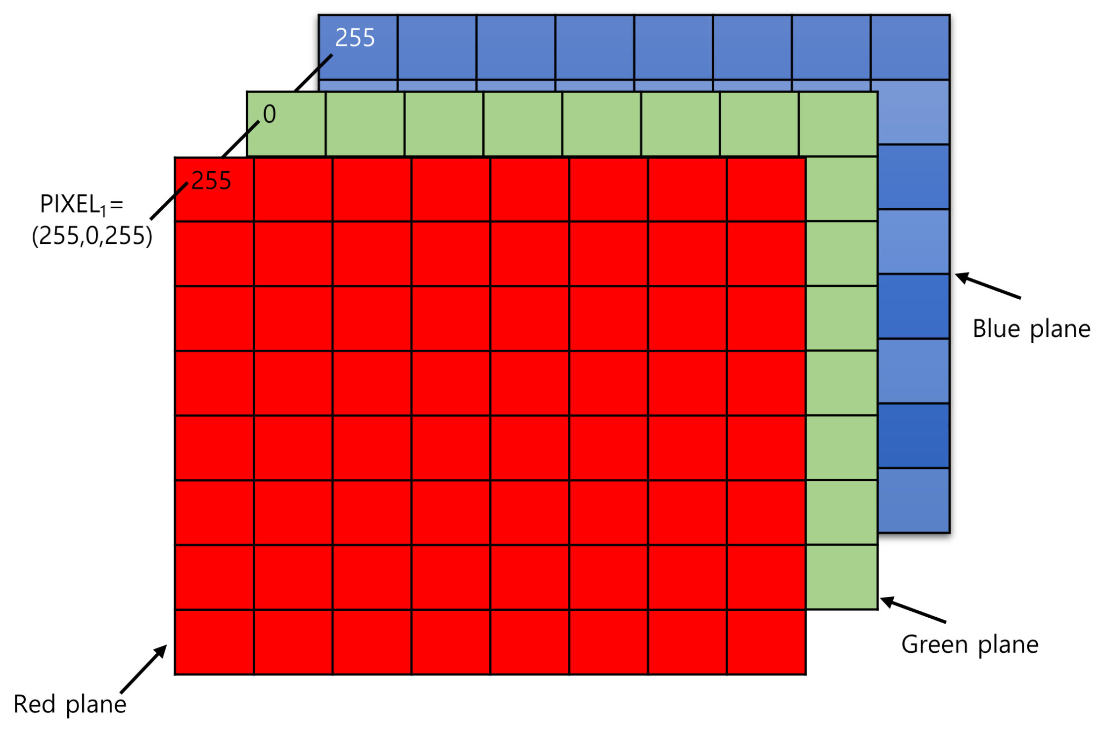
Illustration of tensors of different rank.
Shapes of photos

A photo is a rank 3 tensor.
How we see them

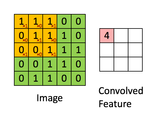
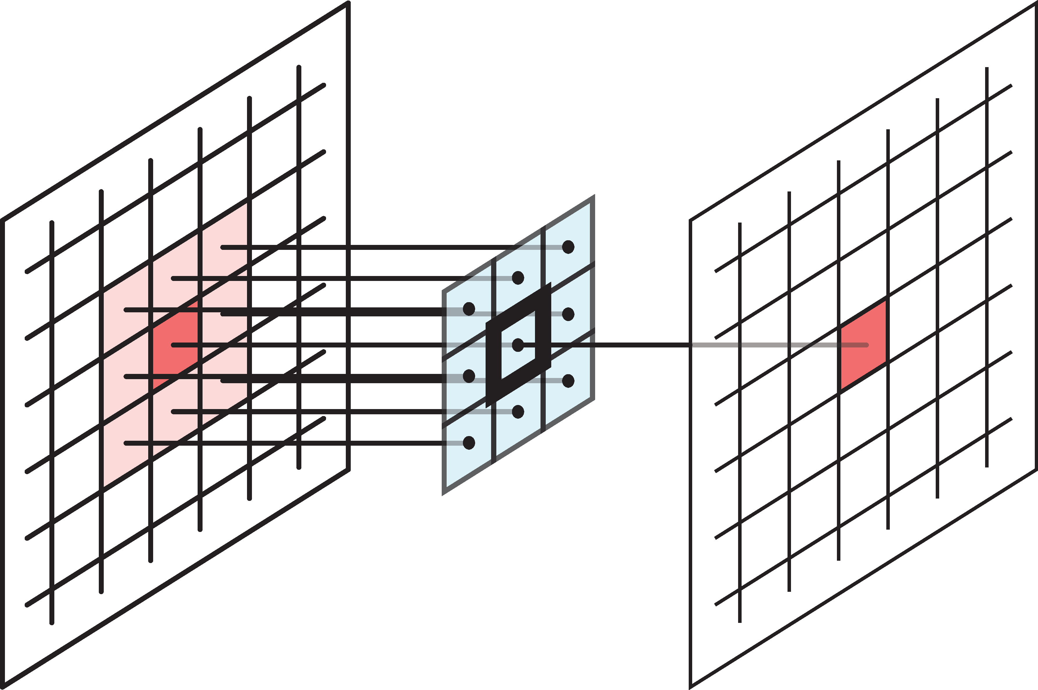
The convolution operation
Scan the 3-channel input (colour image) with the neuron to produce a 1-channel output (grayscale image).
The output is produced by sweeping the neuron over the input. This is called convolution.
Aside: you’d have seen the convolution operation when calculating the density of S = X_1 + X_2 for i.i.d. X_1, X_2 \sim f_X as f_S(s) = \int f_X(x_1)\, f_X(s - x_1)\,\mathrm{d}x_1 = (f_X \star f_X)(s). This is why they’re named “convolutional”.
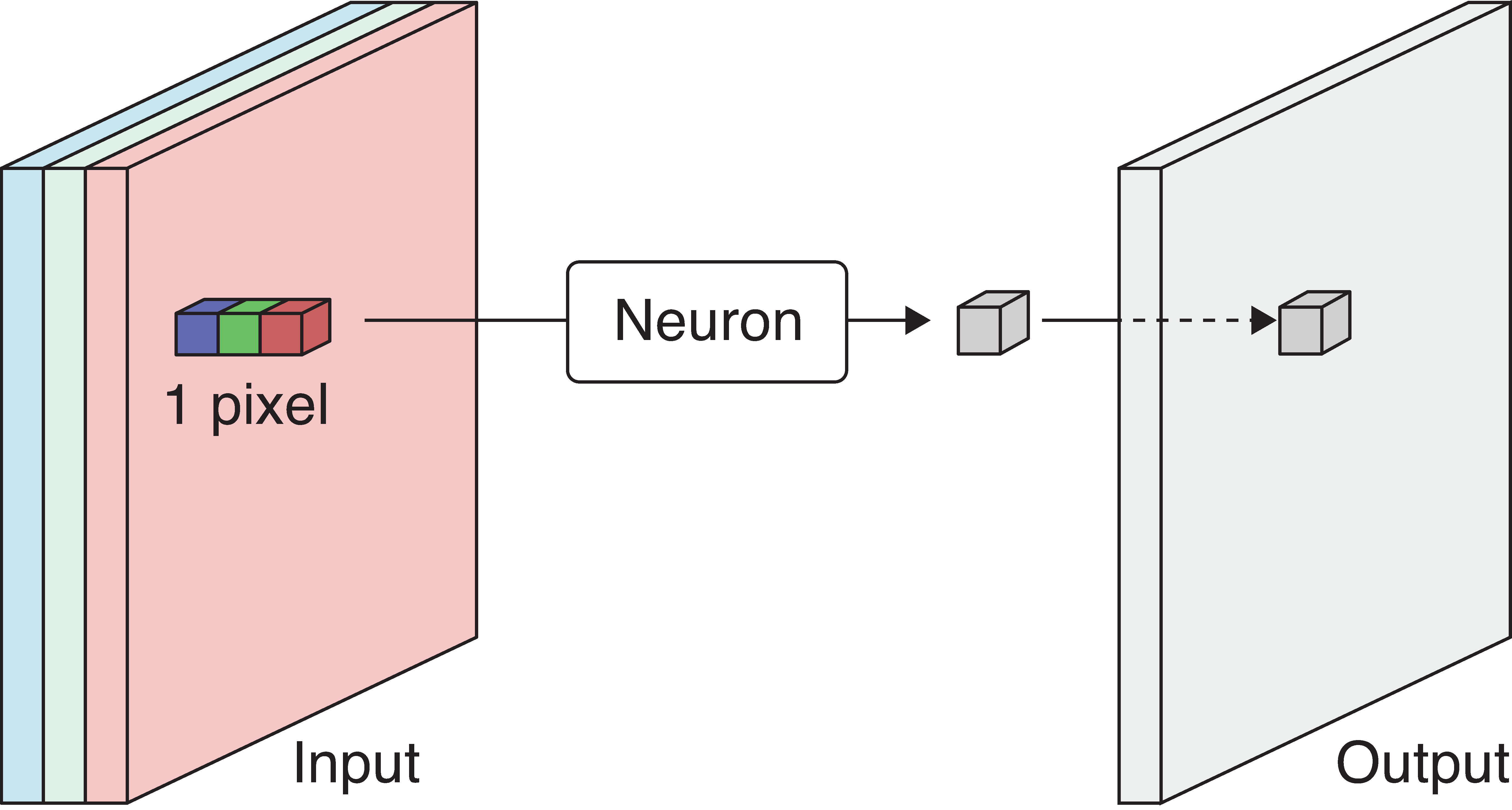
The weights and biases
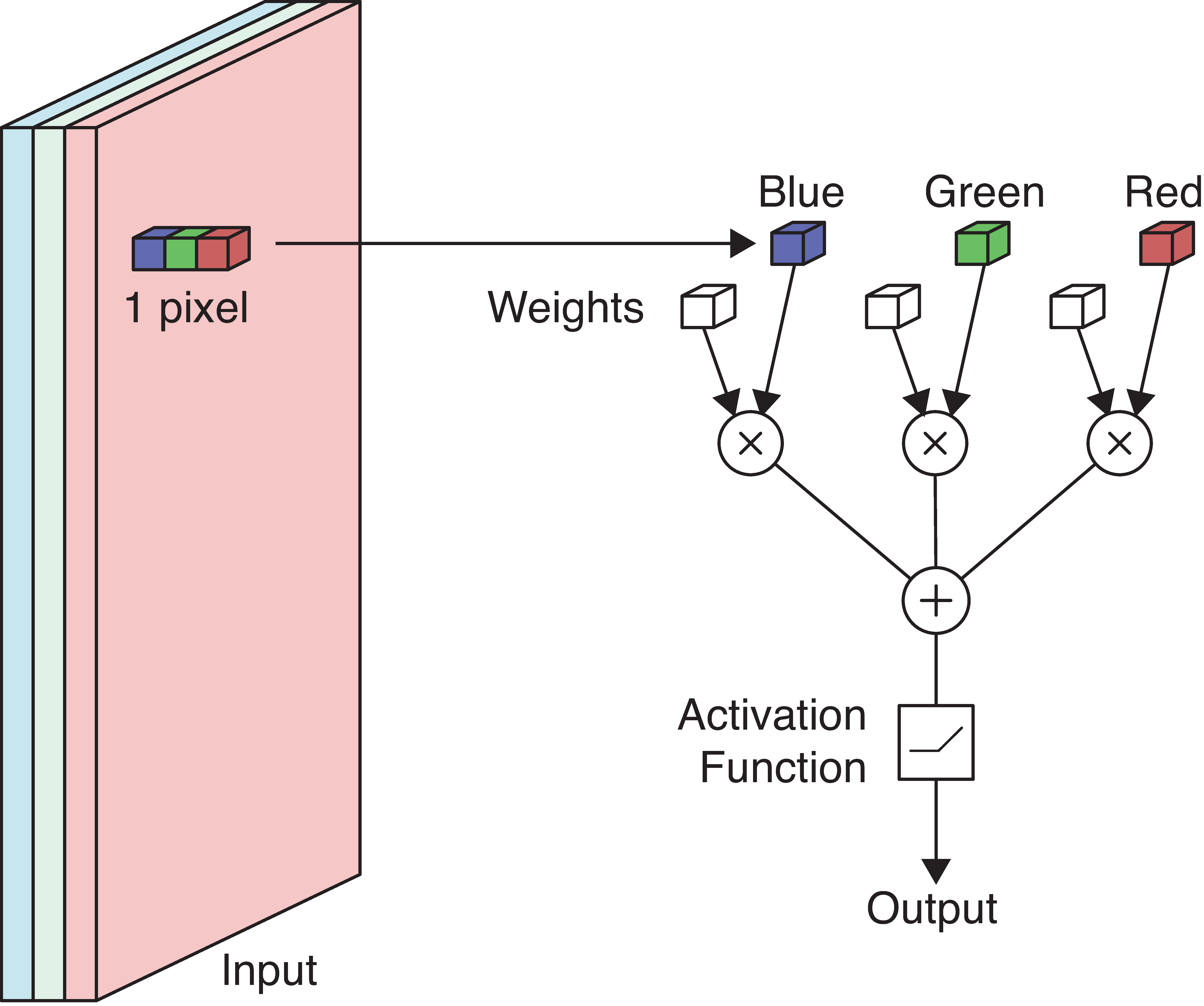
Applying a neuron to an image pixel.
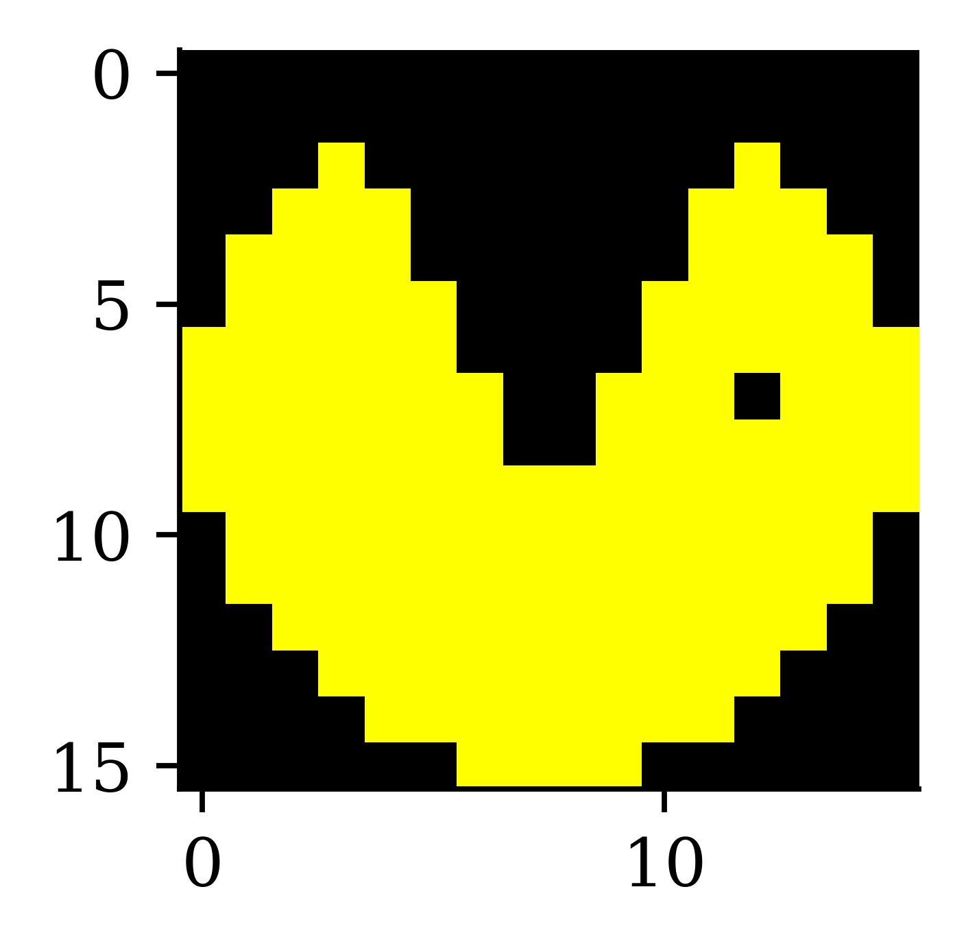
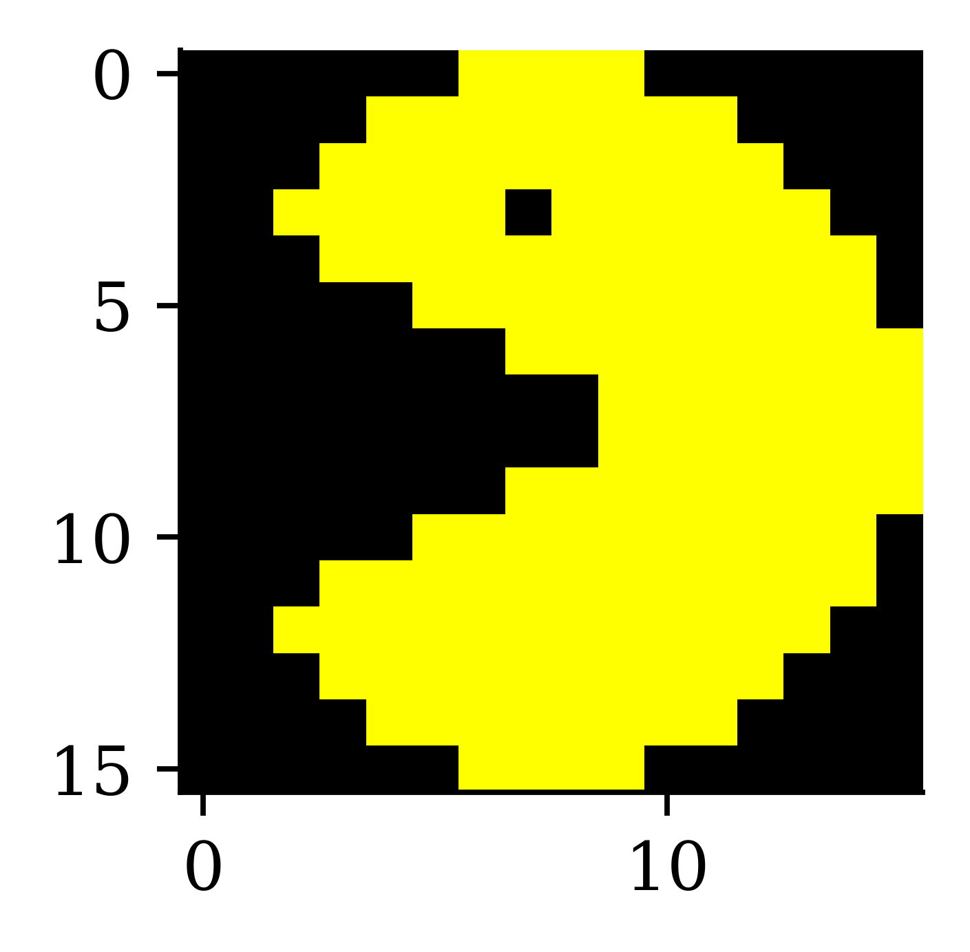
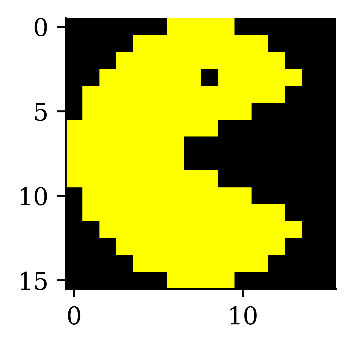
Example: Detecting yellow
If red/green \nearrow or blue \searrow then yellowness \nearrow. Set RGB weights to 1, 1, -1.
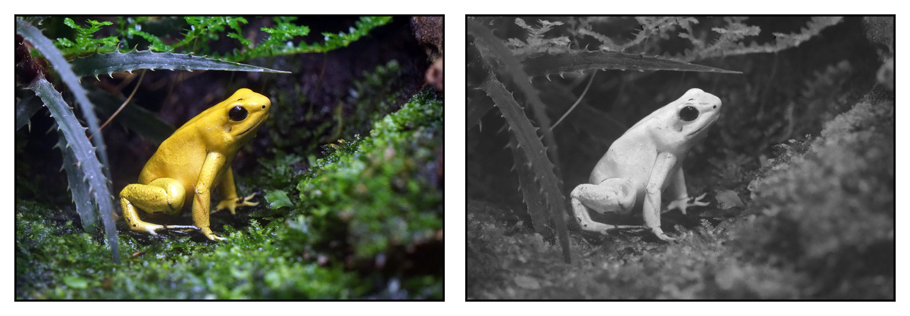
The more yellow the pixel in the colour image (left), the more white it is in the grayscale image.
This is about all we can detect by looking pixel-by-pixel. Typically we look at 3x3 or 5x5 blocks of pixels together.
Filters
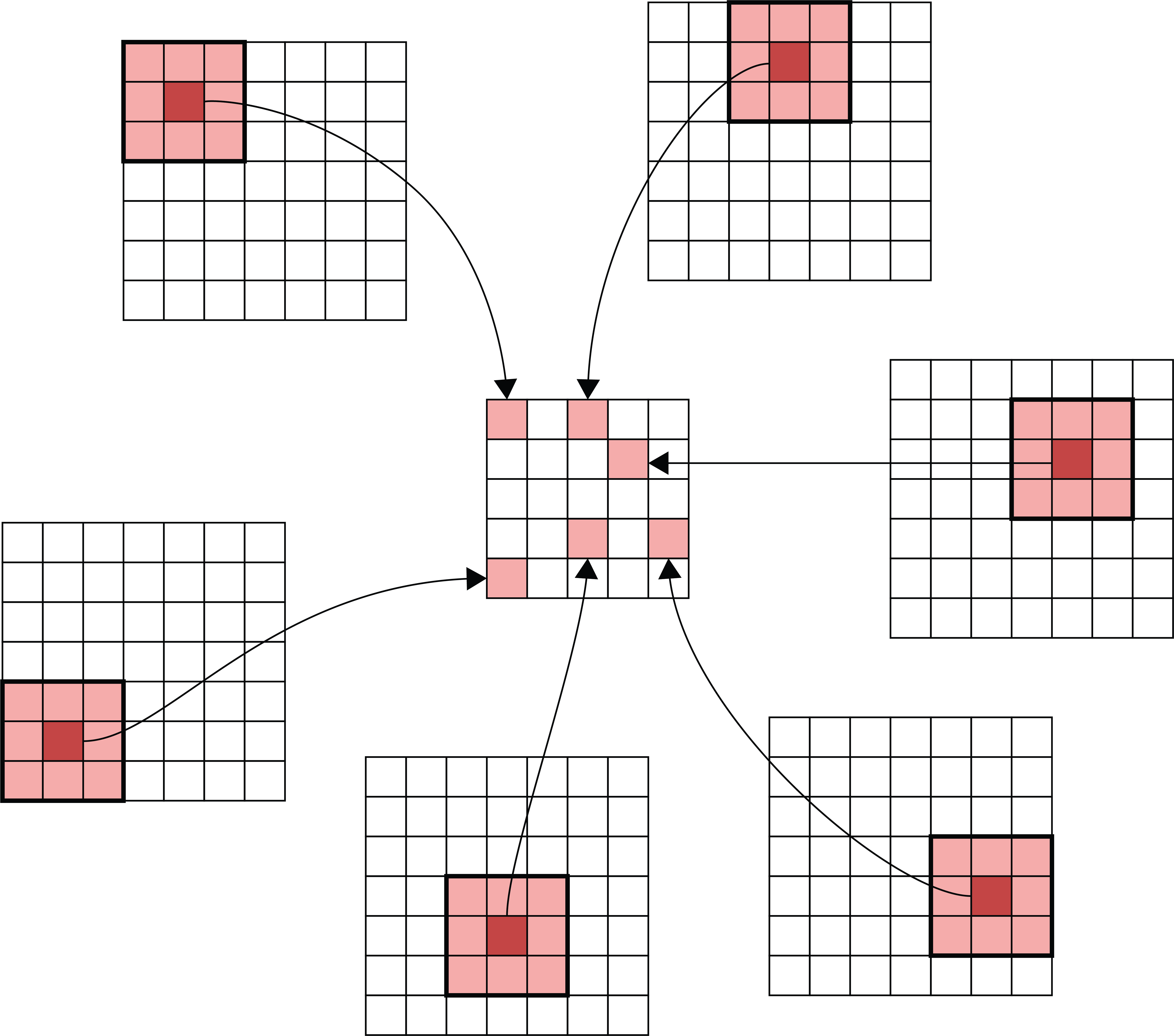
- The patch of input pixels a filter covers at one location is its footprint. Applied there, the filter turns that patch into a single output number — which is exactly what one neuron does.
- The same filter slides over every location instead of learning new weights per pixel. This weight sharing is why a convolution layer has so few parameters.
Example filter
An example of filter convolution in action.
Take a look at https://setosa.io/ev/image-kernels/.
Padding
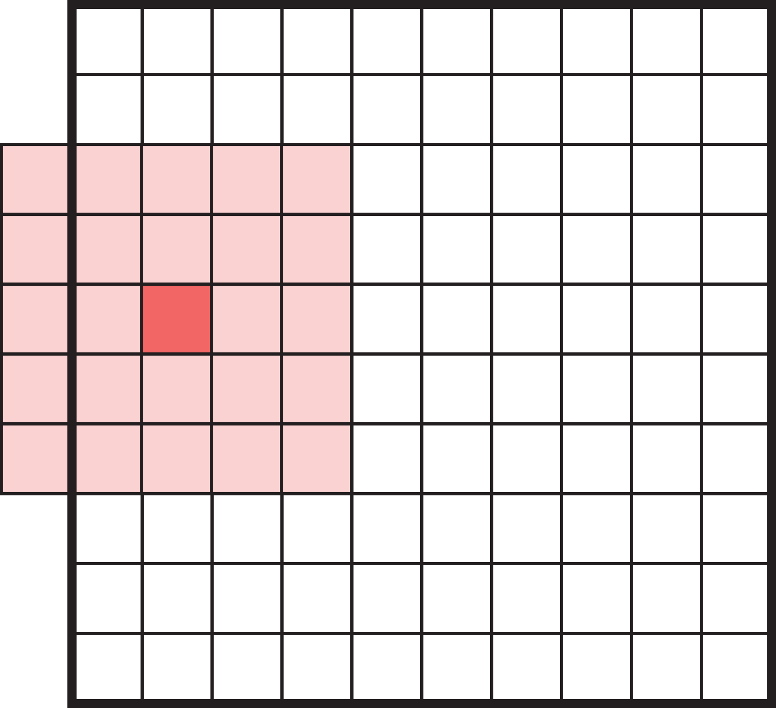
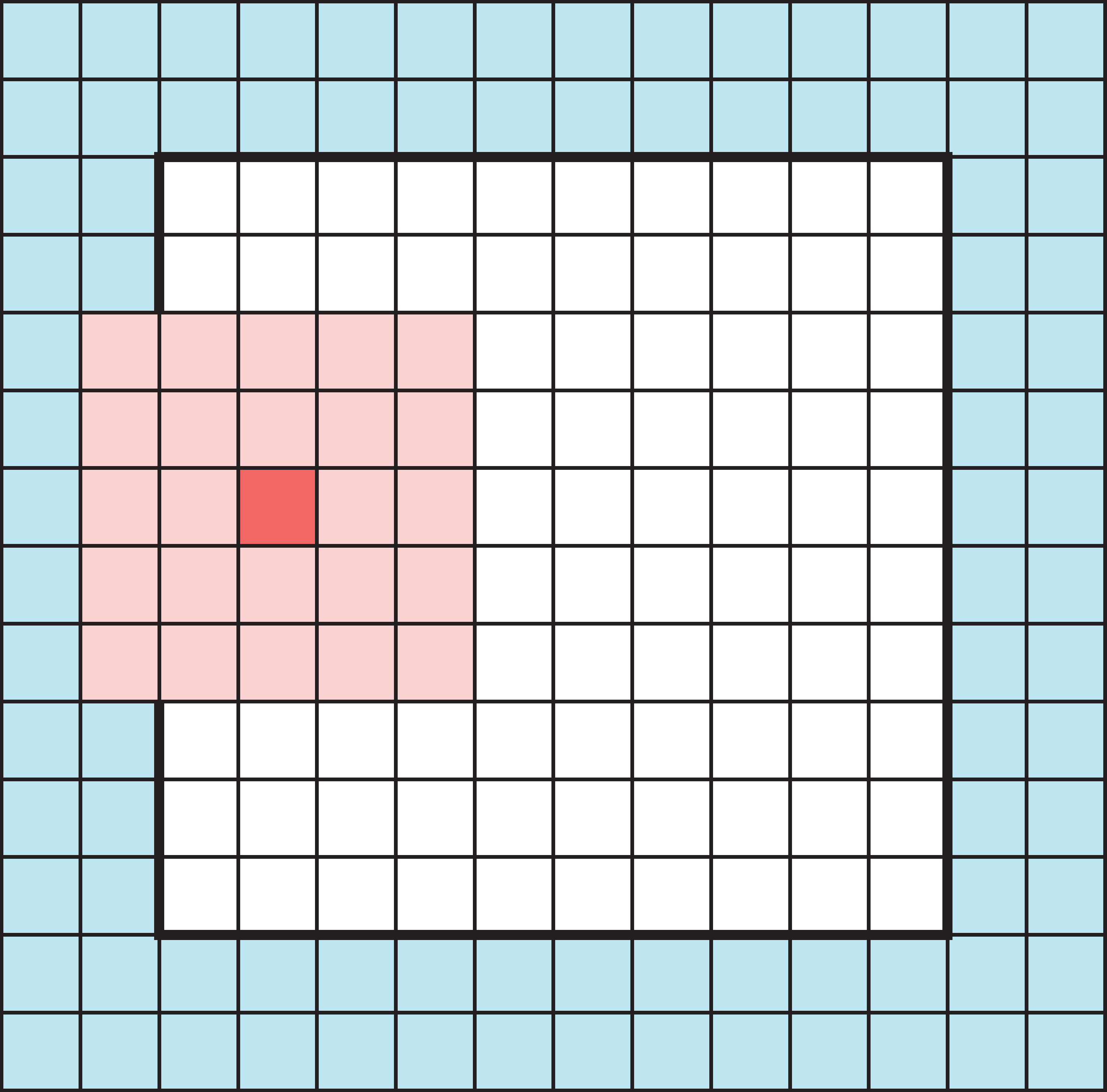
Add zeros around the input so the filter’s footprint doesn’t fall off the edge. This lets the output keep the same size as the input (padding="same").
Striding
We don’t have to move the filter one pixel across/down at a time — a larger stride shrinks the output and saves computation.
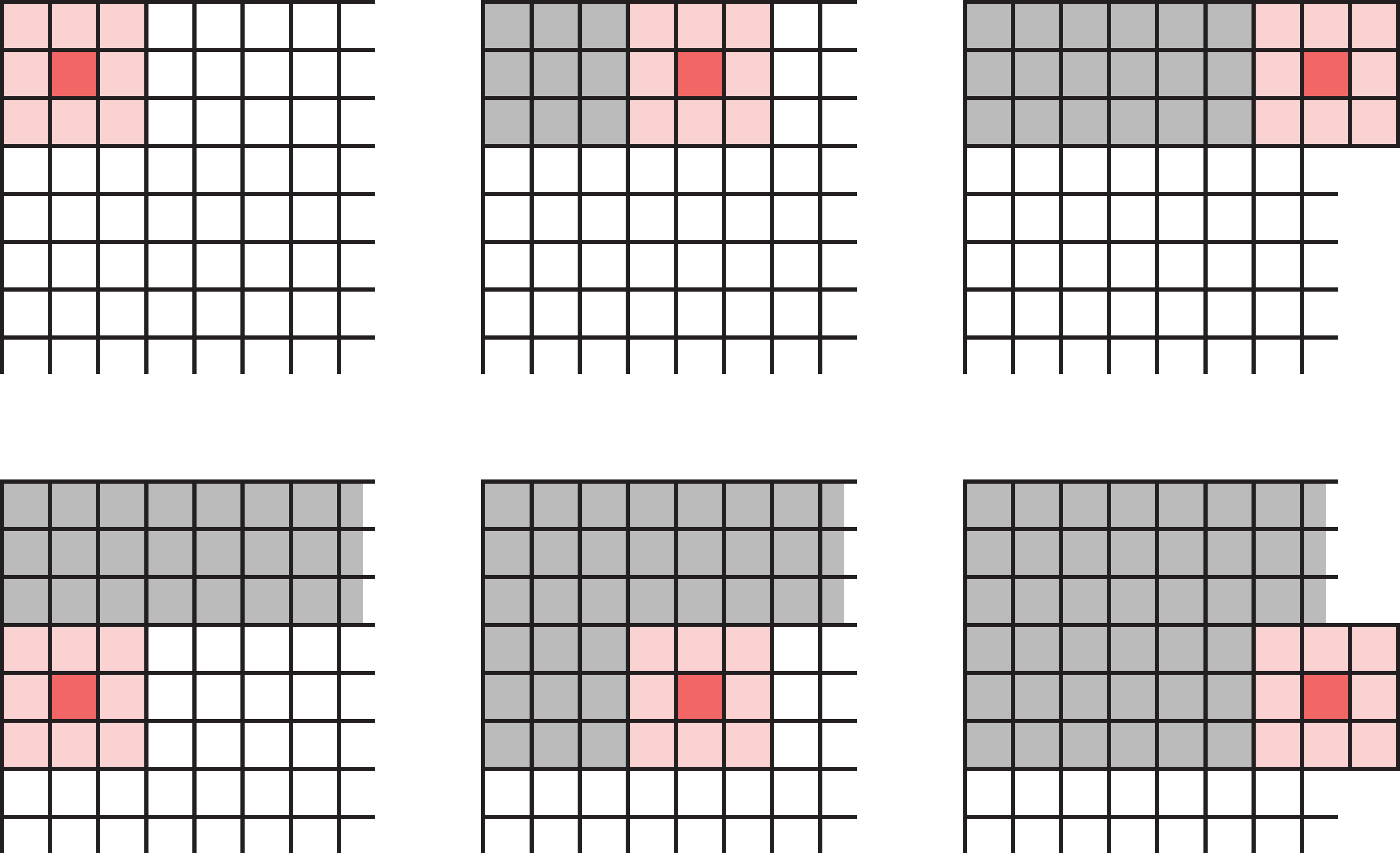
A 3x3 filter with stride 3 in both directions, so no input element is used more than once.
Multidimensional convolution
A filter covers a block of pixels (e.g. a 3x3 filter has 9 weights), and must have the same number of channels as its input.
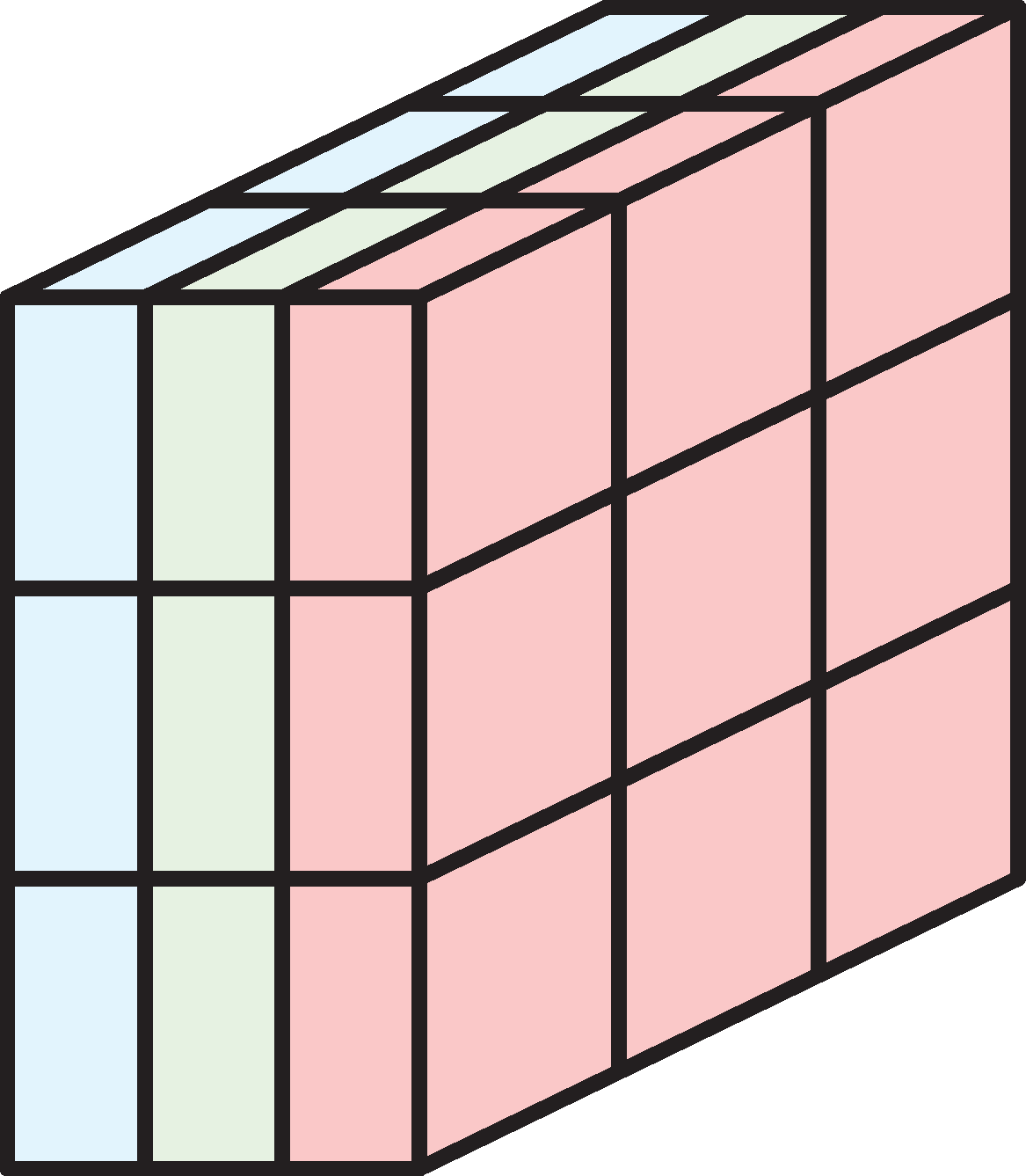
Example: 3x3 filter over RGB input
Each channel is multiplied separately & then added together.
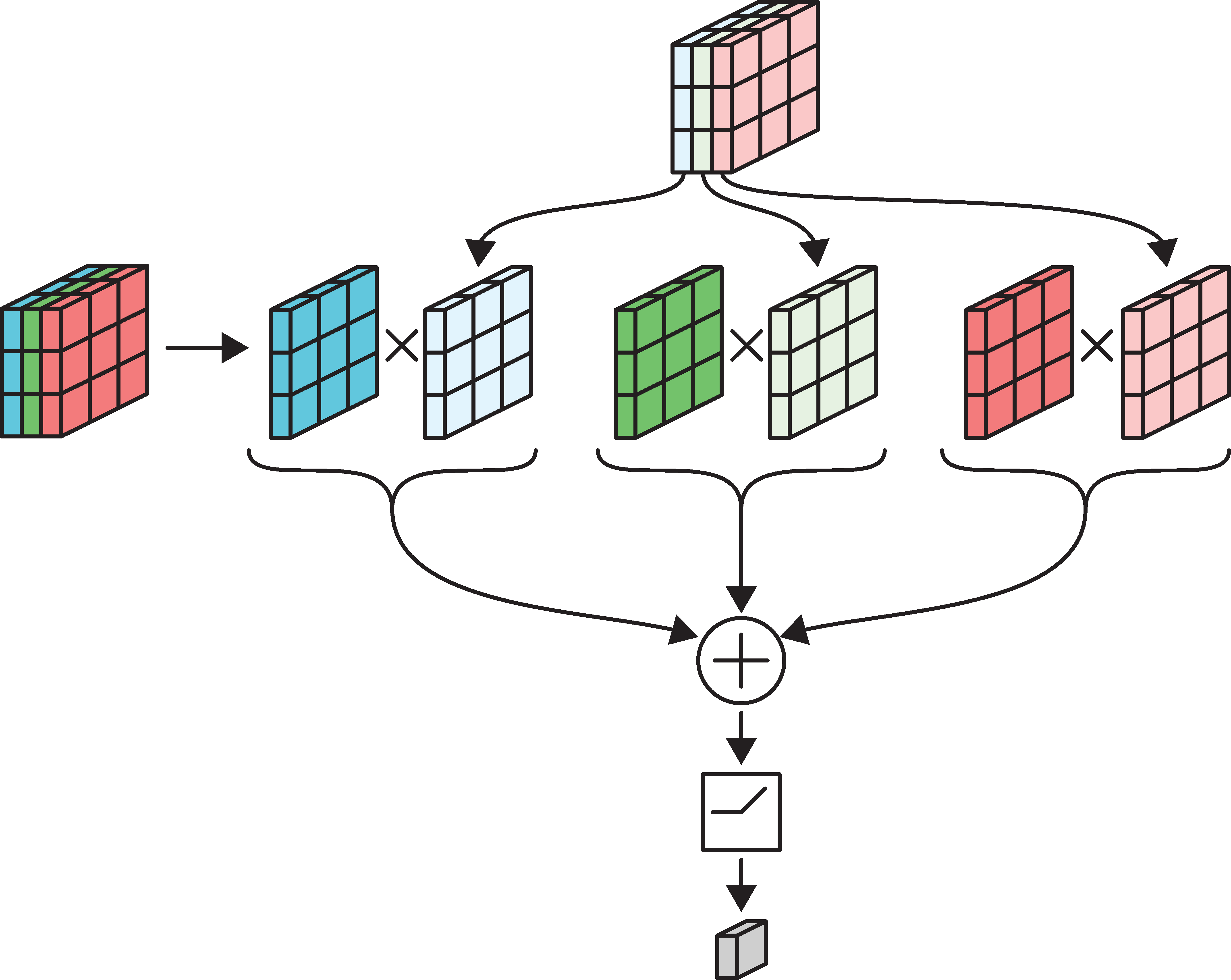
Convolution layer
- Multiple filters are bundled together in one layer.
- The filters are applied simultaneously and independently to the input.
- Number of channels in the output will be the same as the number of filters.
In the image:
- 6-channel input tensor
- input pixels
- four 3x3 filters
- four output tensors
- final output tensor.
Convolutional Neural Networks
A neural network that uses convolution layers is called a convolutional neural network.

A typical CNN structure.
Pooling
Pooling, or downsampling, is a technique to blur a tensor.
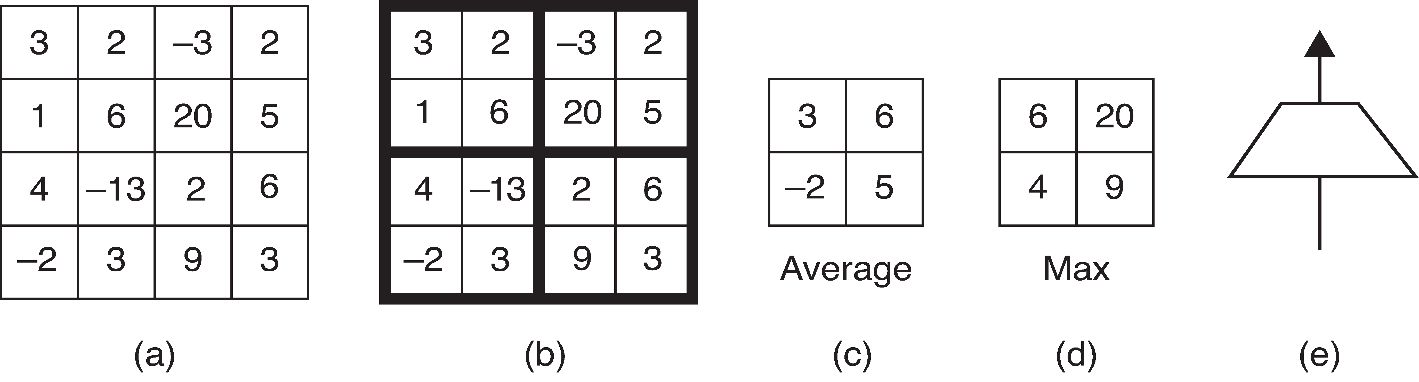
Illustration of pool operations.
(a): Input tensor (b): Subdivide input tensor into 2x2 blocks (c): Average pooling (d): Max pooling (e): Icon for a pooling layer
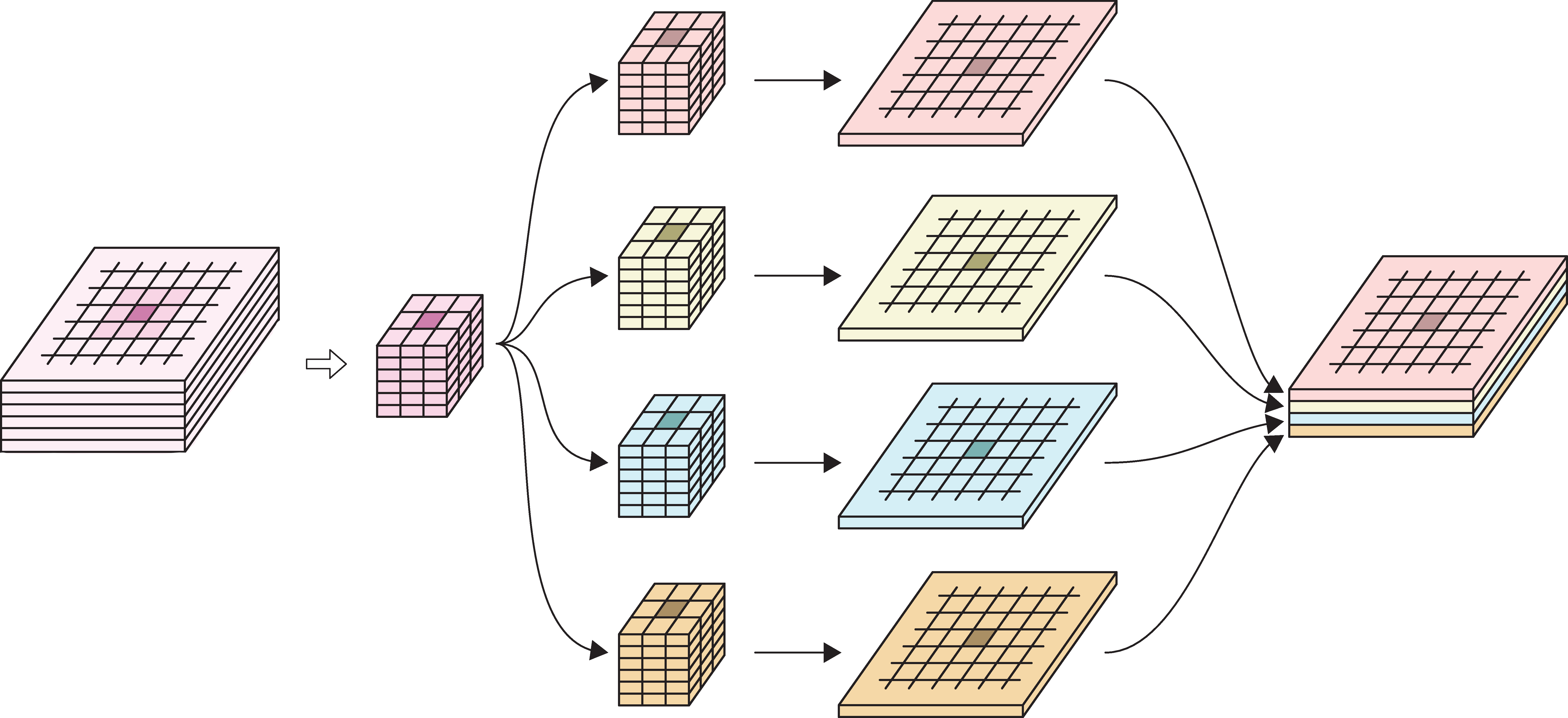
Pooling for multiple channels
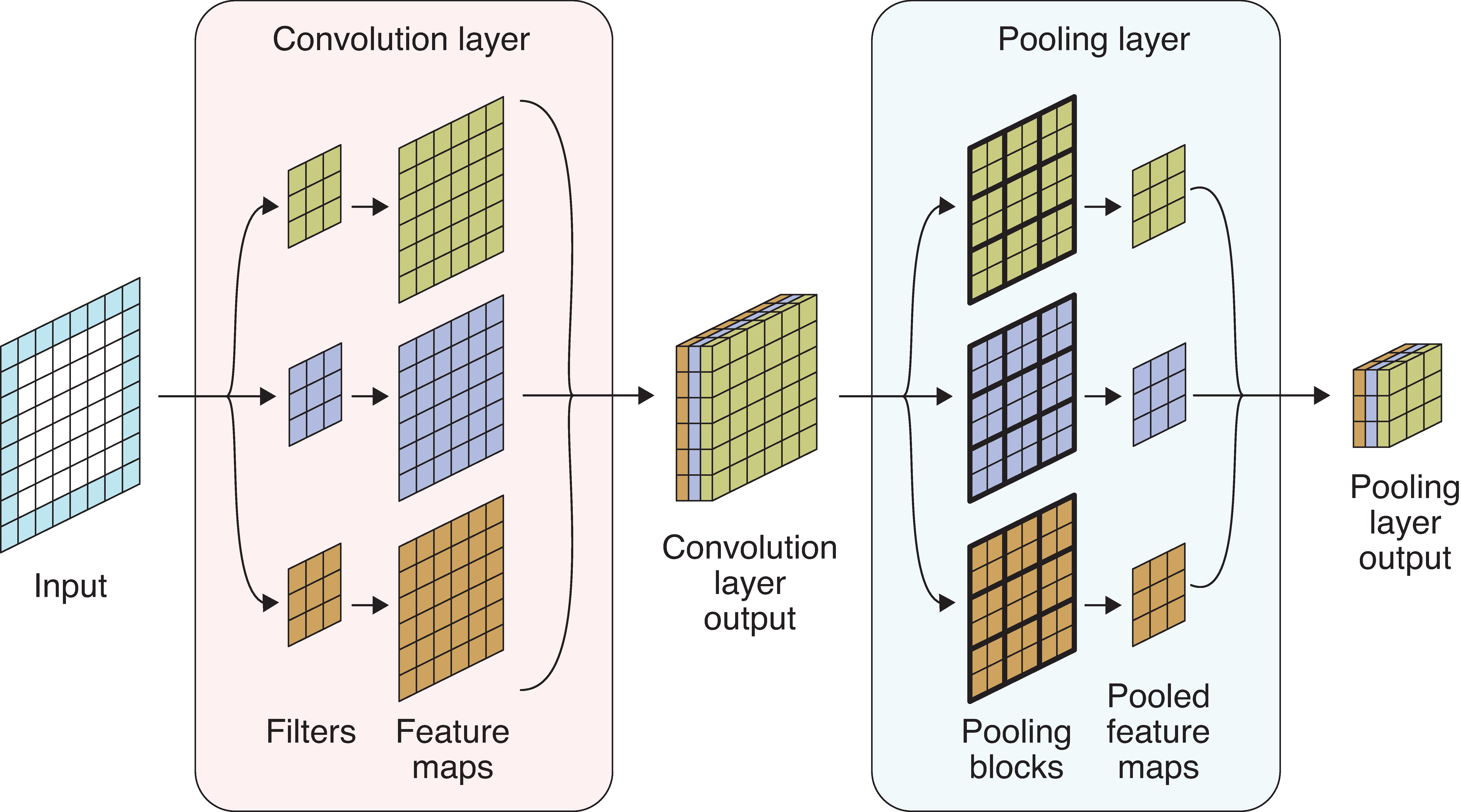
Pooling a multichannel input.
MNIST Dataset
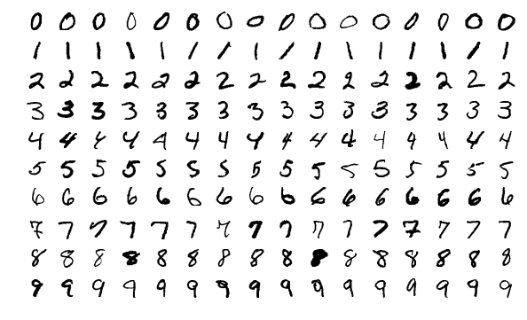
The MNIST dataset.
Depth can be important for image tasks
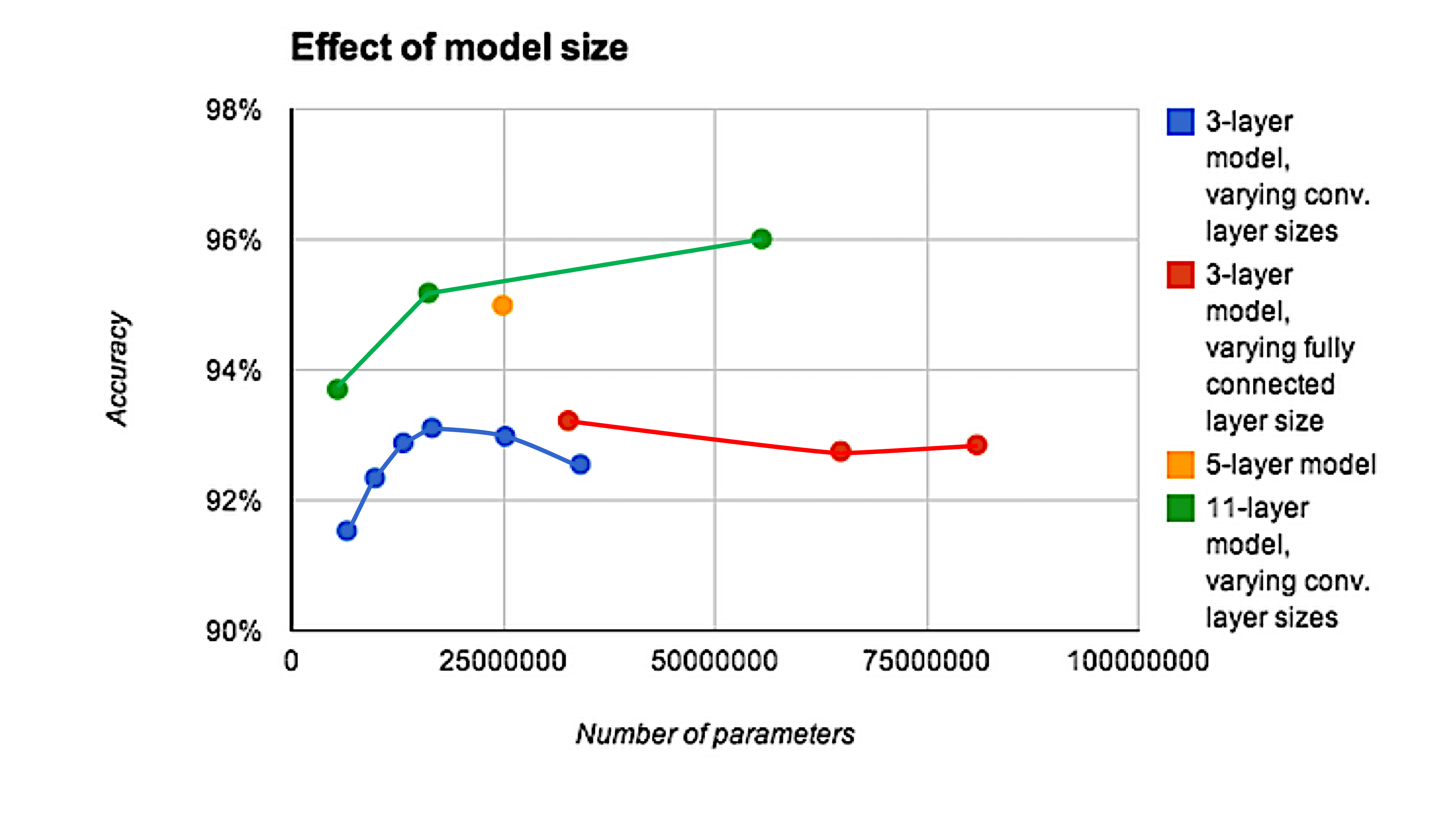
Deeper models aren’t just better because they have more parameters.
Residual connection
Residual (skip) connections (He et al., 2016) let the network learn a correction to the identity, making it possible to train hundreds of layers.
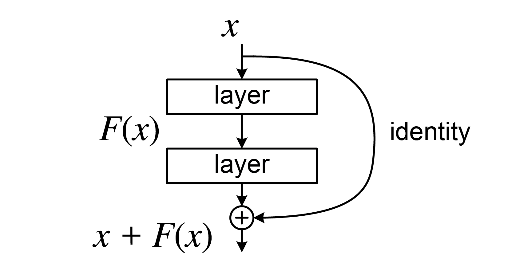
Illustration of a residual connection.
Image augmentation
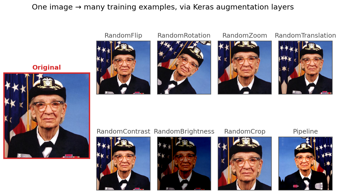
One image becomes many training examples, using Keras’ built-in augmentation layers.
What do the CNN layers learn?
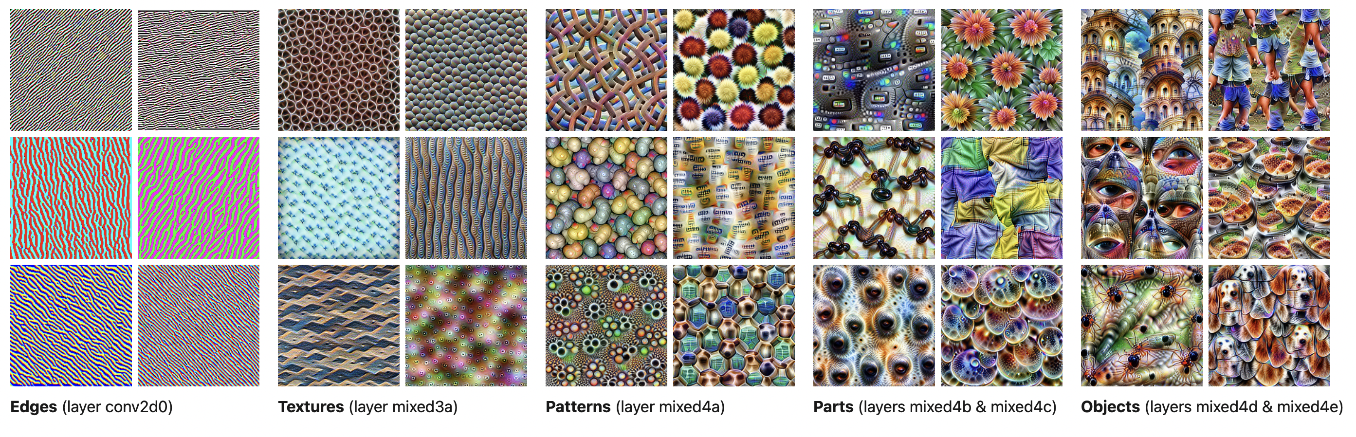
Early layers learn simple patterns; deep layers, complex ones.
How does that work?
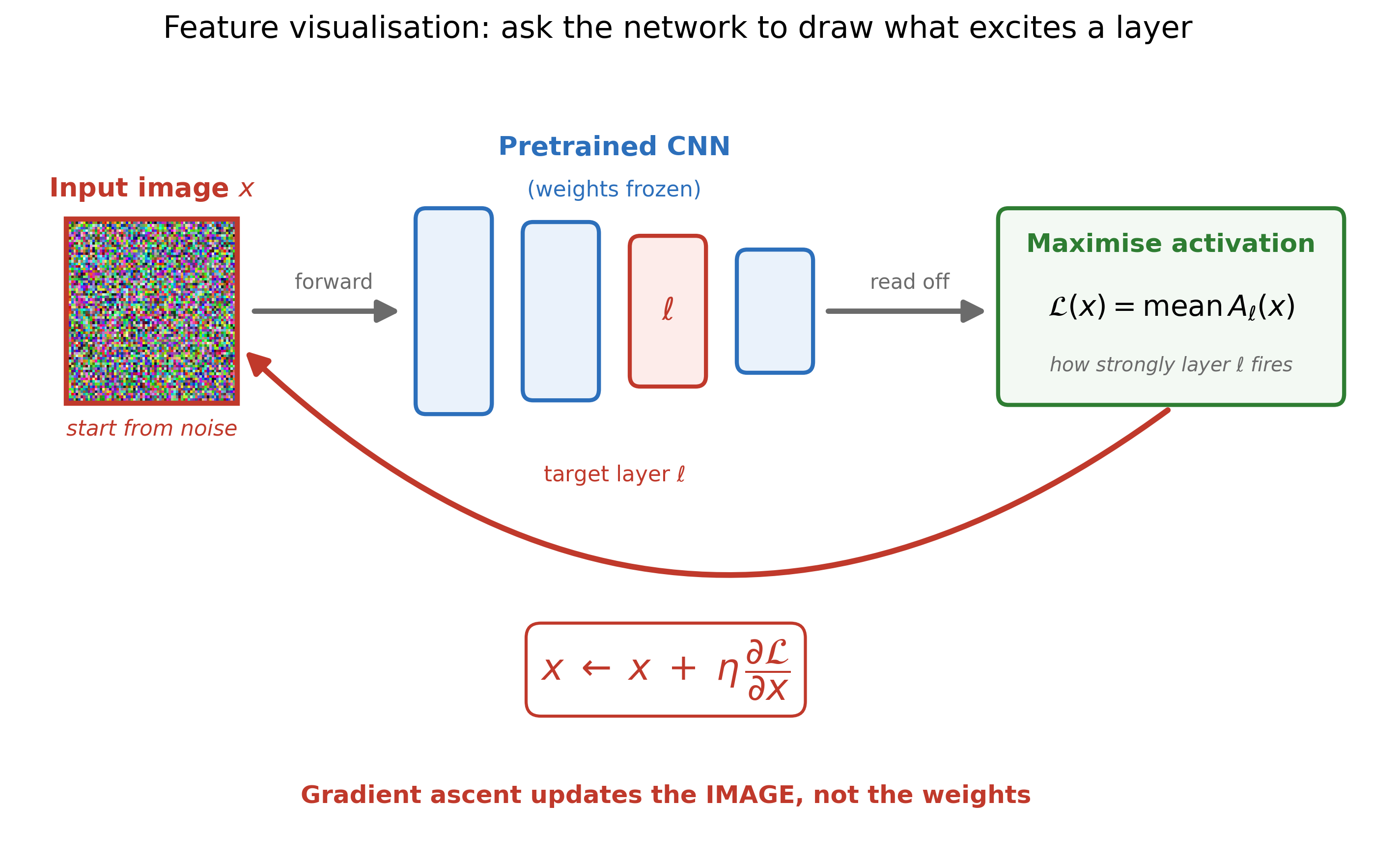
Start from a noise image and nudge its pixels until a chosen layer fires hardest.
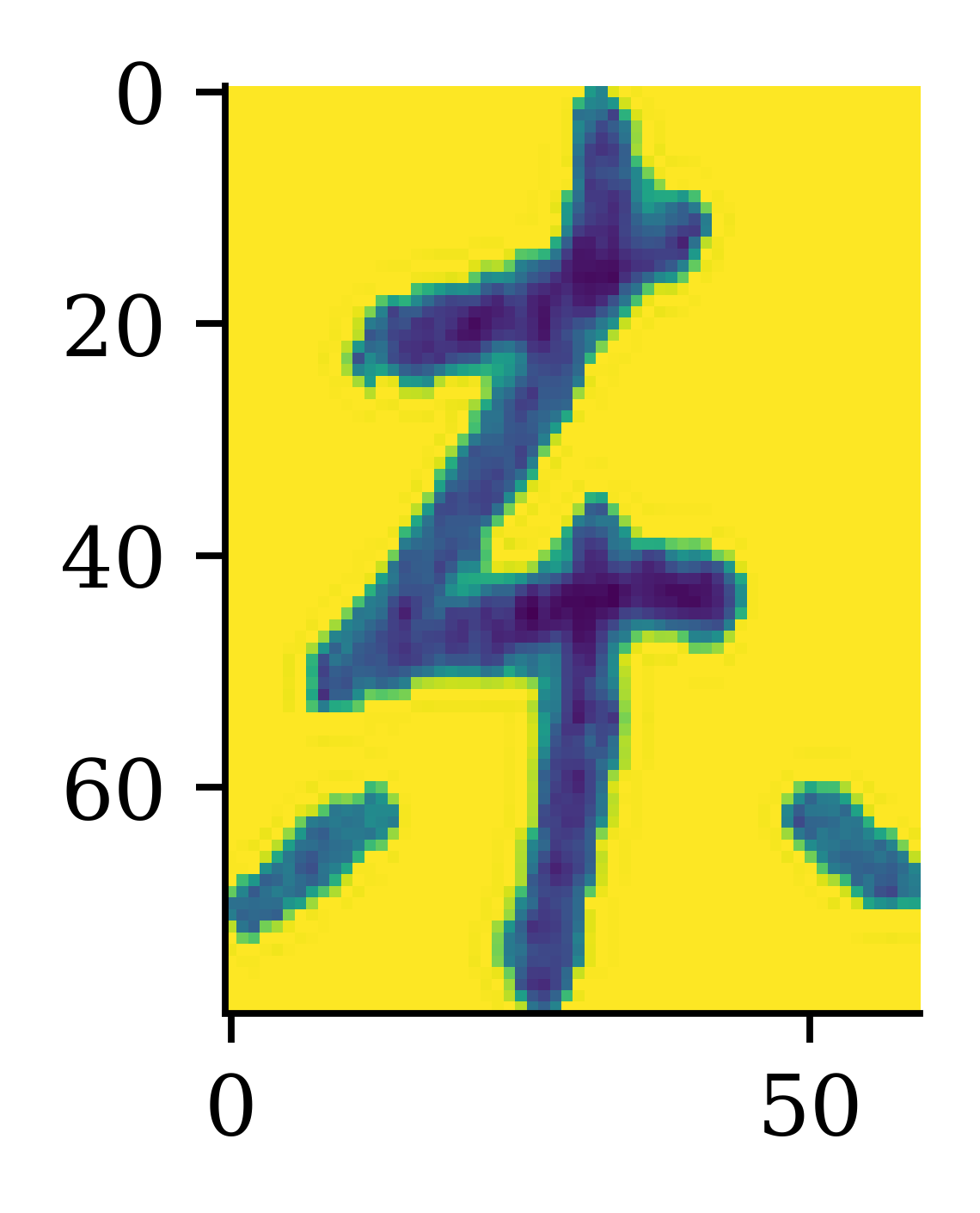
CASIA Chinese handwriting database
Dataset source: Institute of Automation of Chinese Academy of Sciences (CASIA)
A 13 GB dataset of 3,999,571 handwritten characters.
Number of images for each character
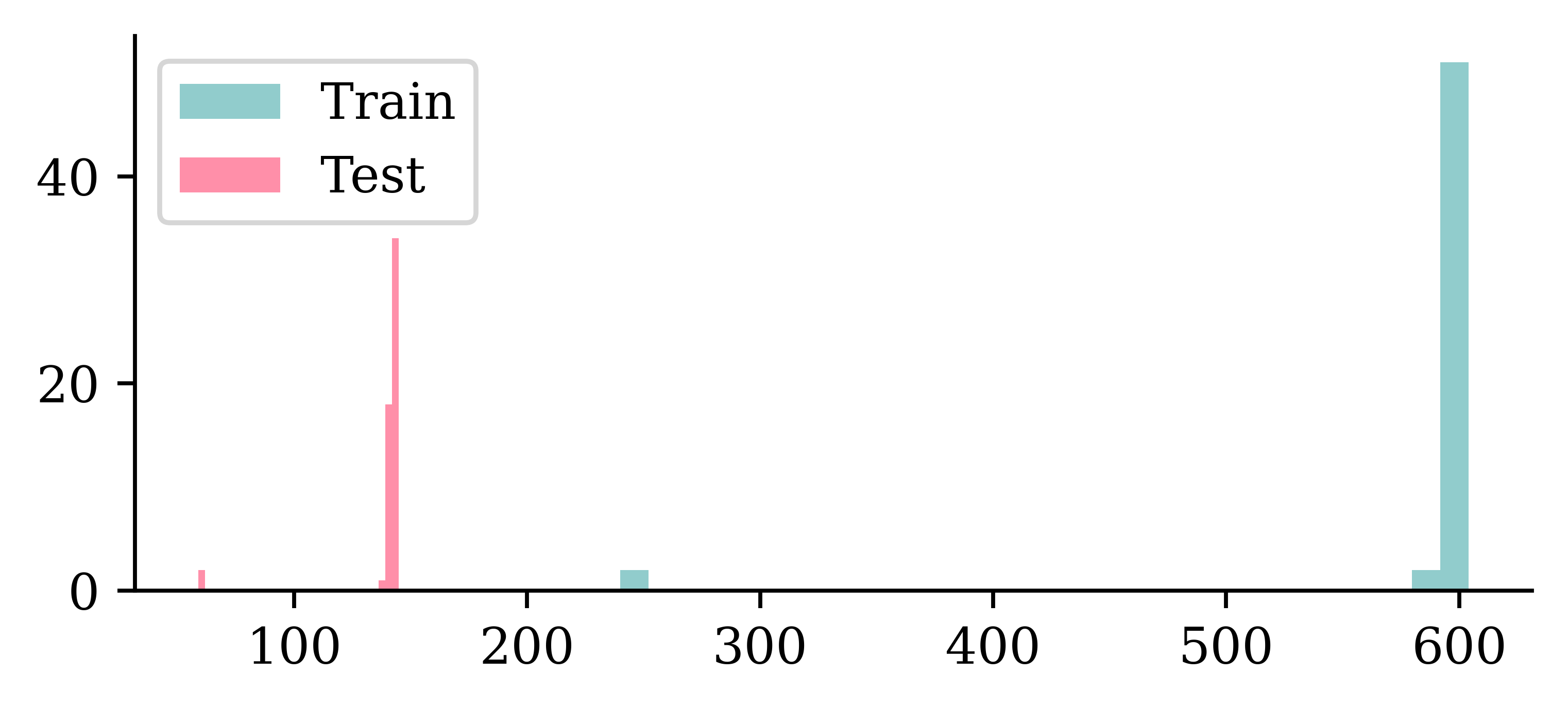
It differs, but basically ~600 training and ~140 test images per character. A couple of characters have a lot less of both though.
Checking the dimensions
Code
def get_image_dimensions(root_folder):
    dimensions = []
    for folder in root_folder.glob("*/"):
        for image in folder.glob("*.png"):
            img = imread(image)
            dimensions.append(img.shape)
    return dimensions

train_dimensions = get_image_dimensions(Path("CASIA-Dataset/Train"))
test_dimensions = get_image_dimensions(Path("CASIA-Dataset/Test"))

train_heights = [d[0] for d in train_dimensions]
train_widths = [d[1] for d in train_dimensions]
test_heights = [d[0] for d in test_dimensions]
test_widths = [d[1] for d in test_dimensions]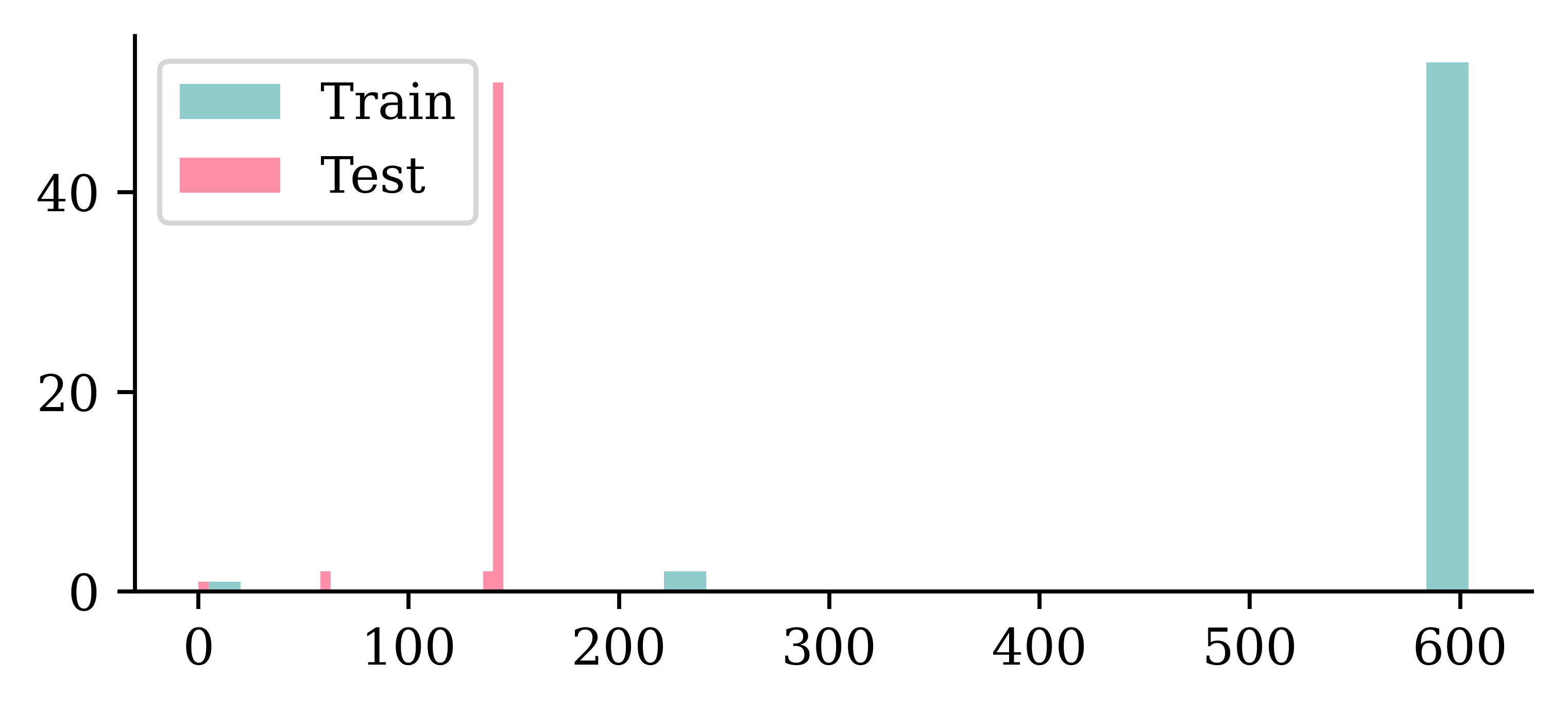
Checking the dimensions II
Using density=True removes the count imbalance, so we can compare the shapes of the distributions.
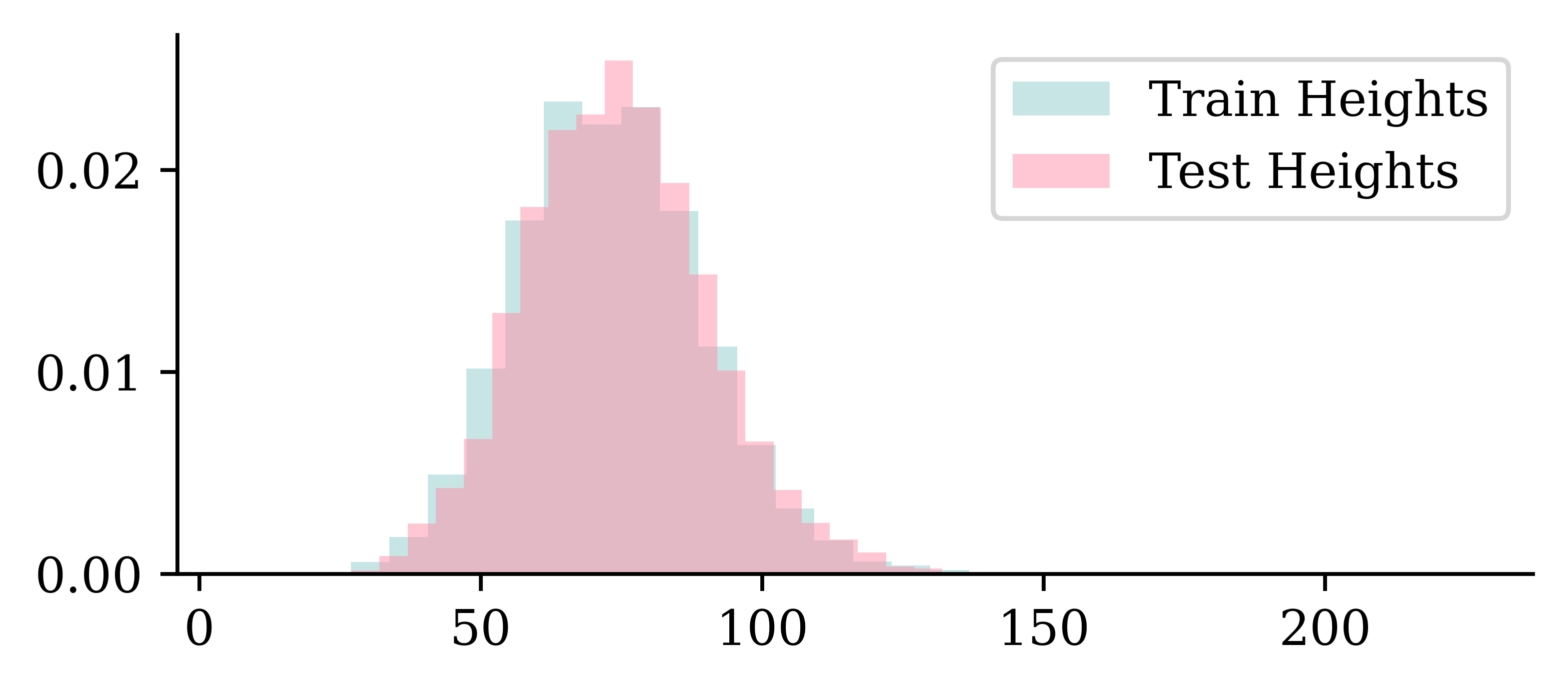
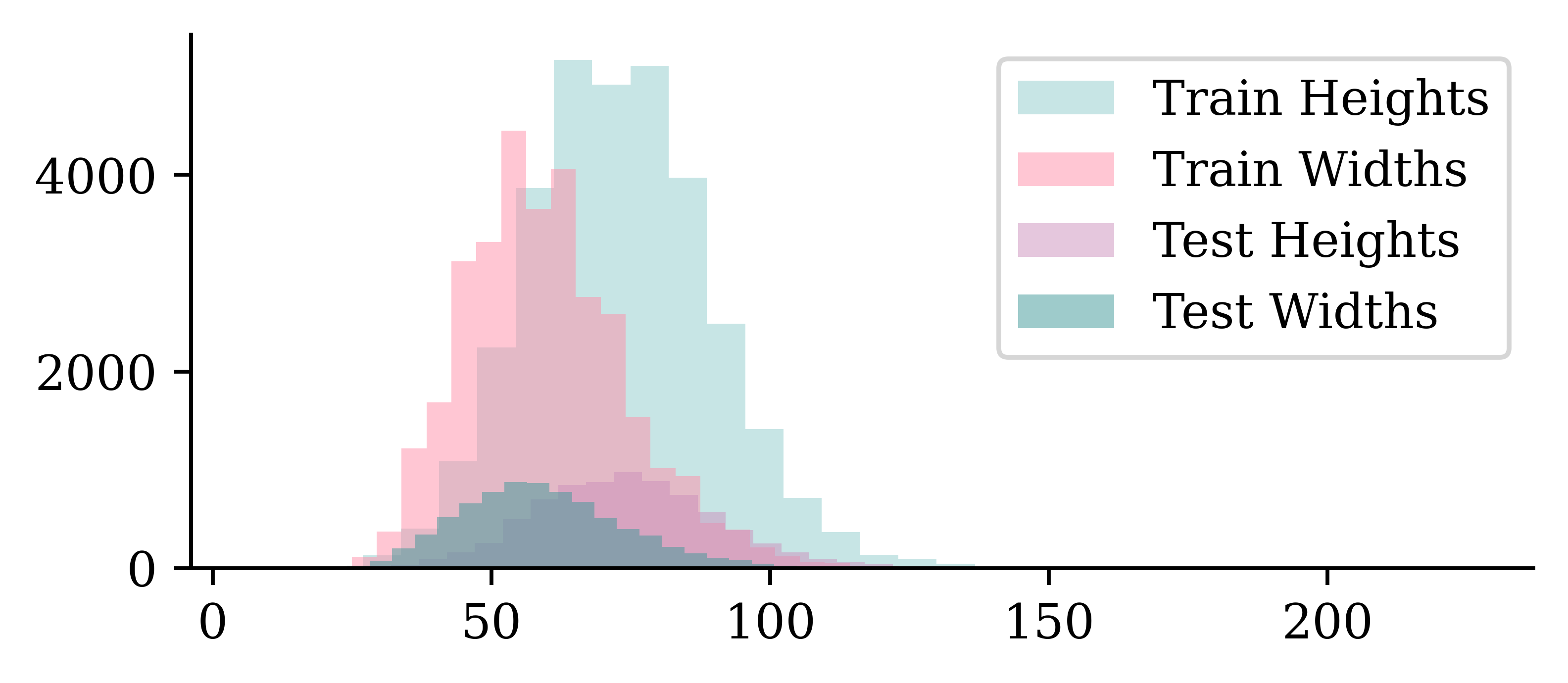
- The images are taller than they are wide.
- The distribution of dimensions is pretty similar between training and test sets.
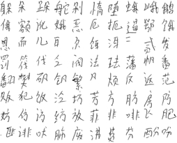
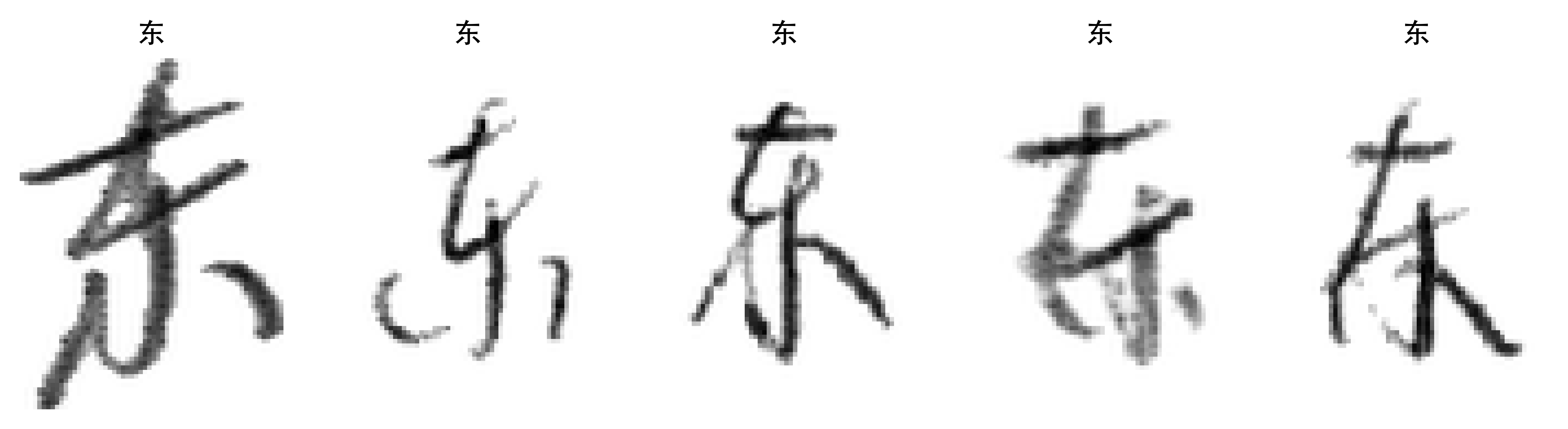
Plotting some training characters

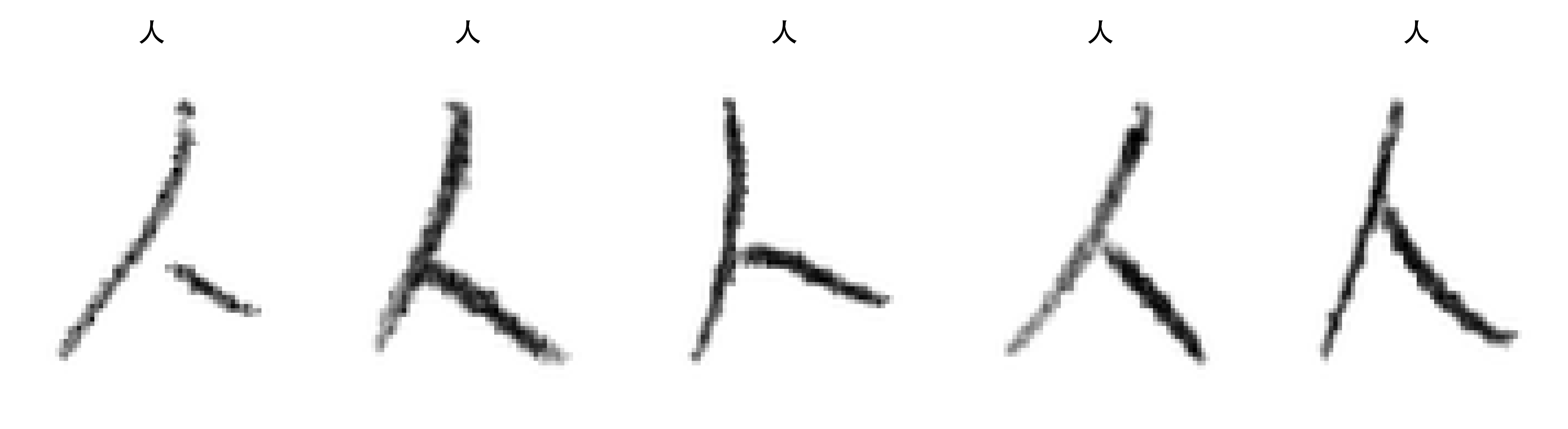
Without the colourmap..
Make simple baseline (multinomial) logistic regression
Basically pretend it’s not an image
Tip
The Rescaling layer will rescale the intensities to [0, 1].
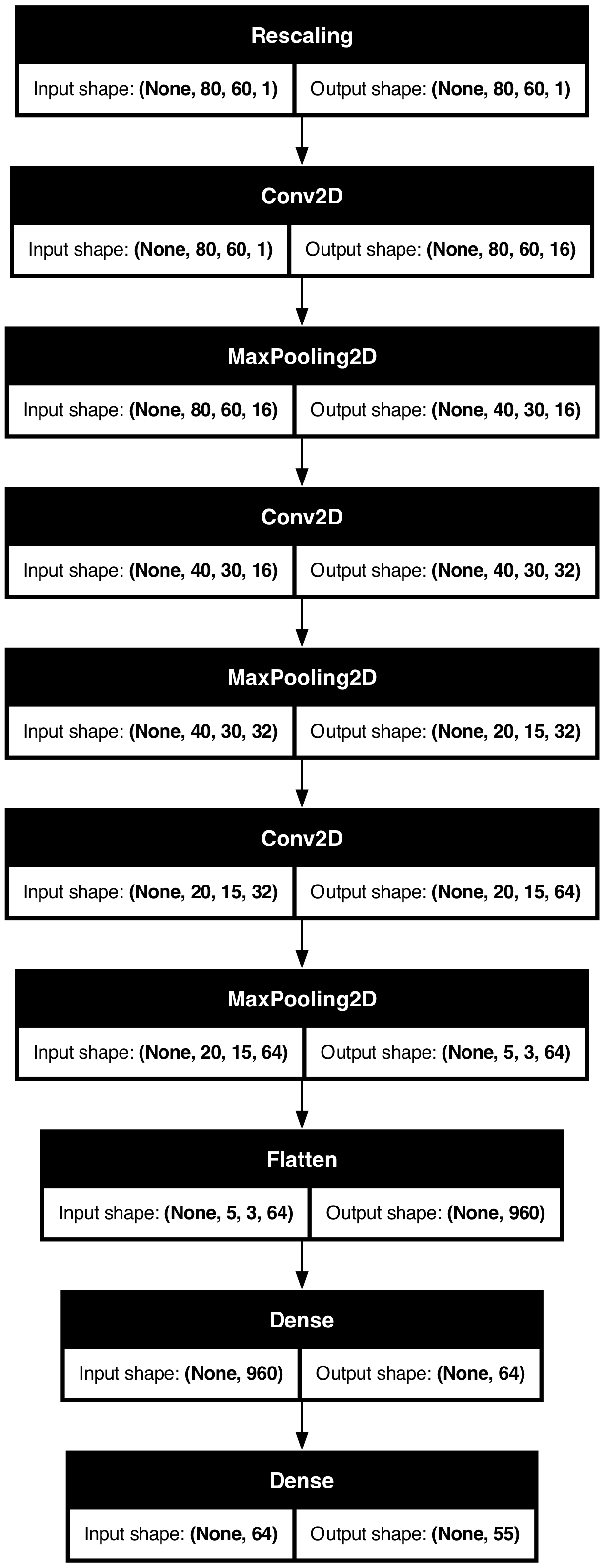
Plot the model
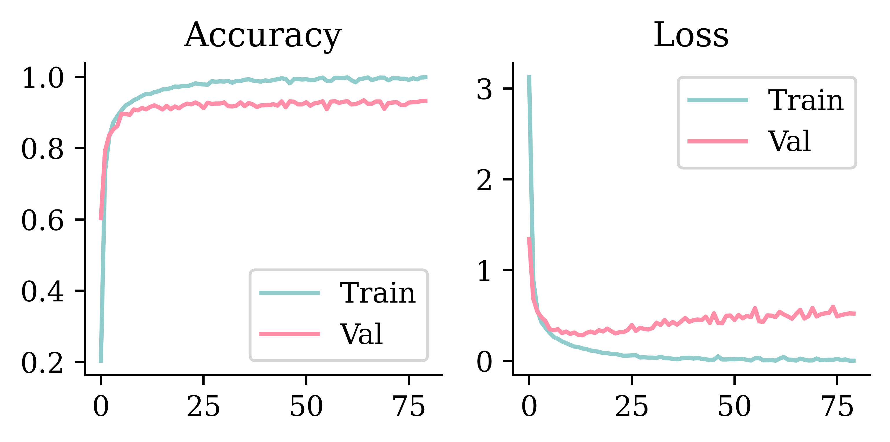
Plot the loss/accuracy curves
Code
def plot_history(history):
    epochs = range(len(history["loss"]))

    plt.subplot(1, 2, 1)
    plt.plot(epochs, history["accuracy"], label="Train")
    plt.plot(epochs, history["val_accuracy"], label="Val")
    plt.legend(loc="lower right")
    plt.title("Accuracy")

    plt.subplot(1, 2, 2)
    plt.plot(epochs, history["loss"], label="Train")
    plt.plot(epochs, history["val_loss"], label="Val")
    plt.legend(loc="upper right")
    plt.title("Loss")
    plt.show()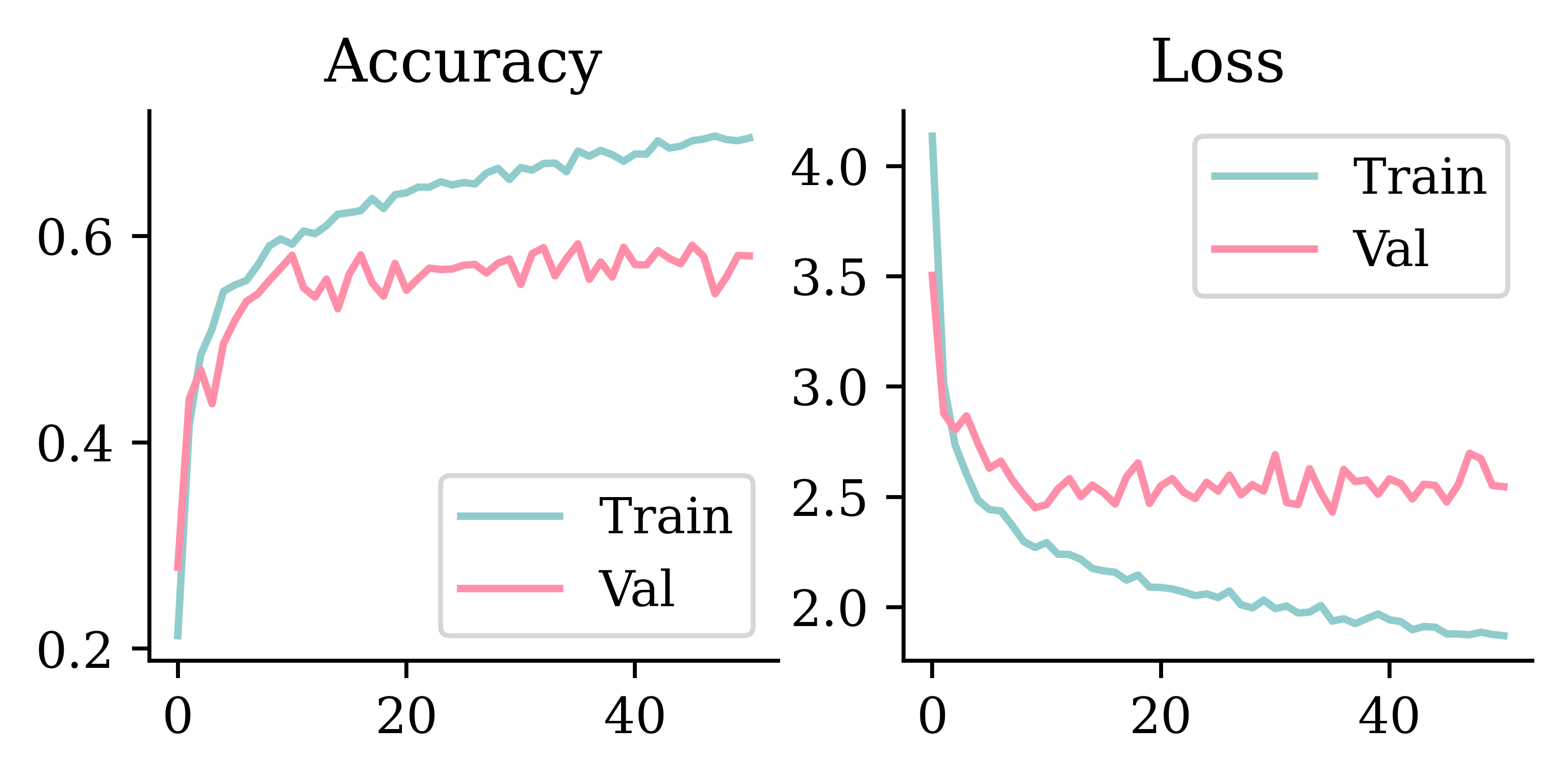
Plot the CNN
Plot the loss/accuracy curves
Predict on the test set II

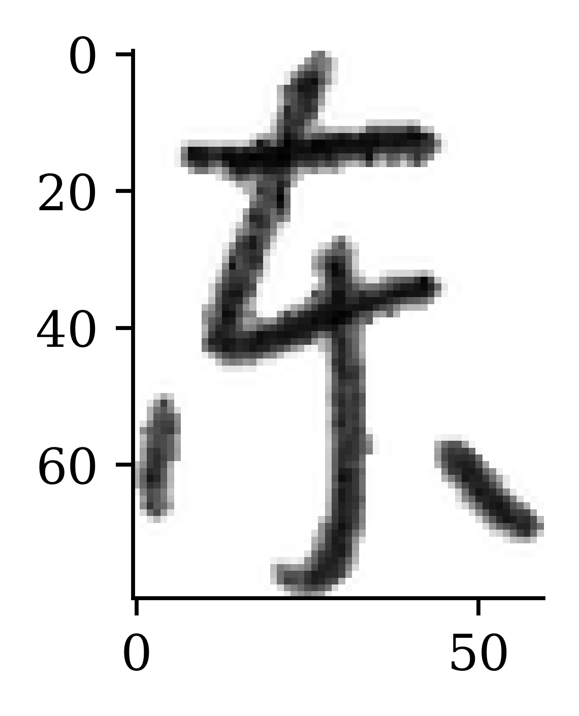
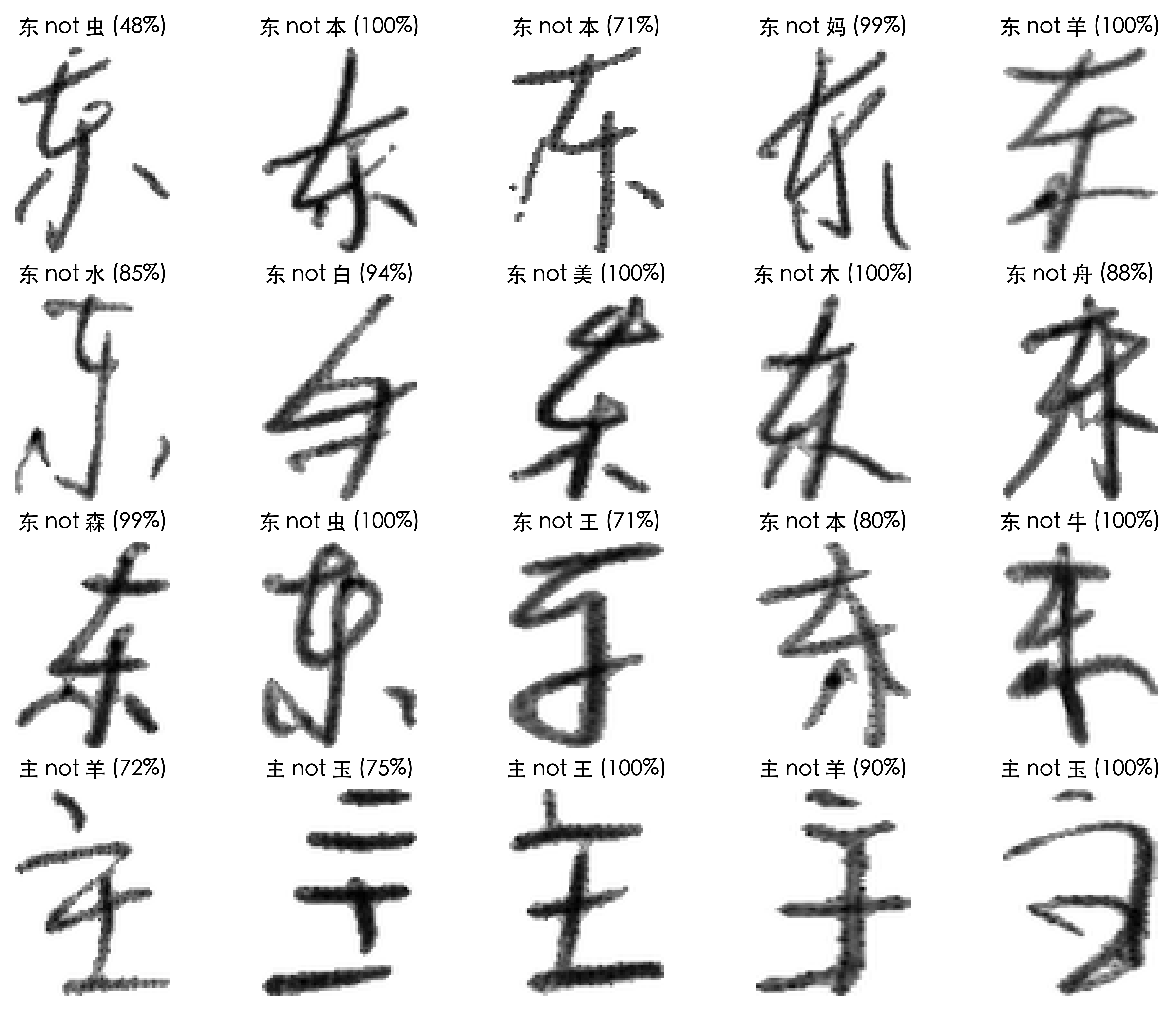
Take a look at the failure cases
Code
def plot_failed_predictions(X, y, class_names, max_errors = 20,
            num_rows = 2, num_cols = 5, title_font=CHINESE_FONT):
    plt.figure(figsize=(num_cols * 2, num_rows * 2))
    errors = 0
    y_pred = model.predict(X, verbose=0)
    y_pred_classes = y_pred.argmax(axis=1)
    y_pred_probs = keras.ops.convert_to_numpy(keras.ops.softmax(y_pred)).max(axis=1)
    for i in range(len(y_pred)):
        if errors >= min(max_errors, num_rows * num_cols):
            break
        if y_pred_classes[i] != y[i]:
            plt.subplot(num_rows, num_cols, errors + 1)
            plt.imshow(X[i], cmap="gray")
            true_class = class_names[y[i]]
            pred_class = class_names[y_pred_classes[i]]
            conf = y_pred_probs[i]
            msg = f"{true_class} not {pred_class} ({conf*100:.0f}%)"
            plt.title(msg, fontproperties=title_font)
            plt.axis("off")
            errors += 1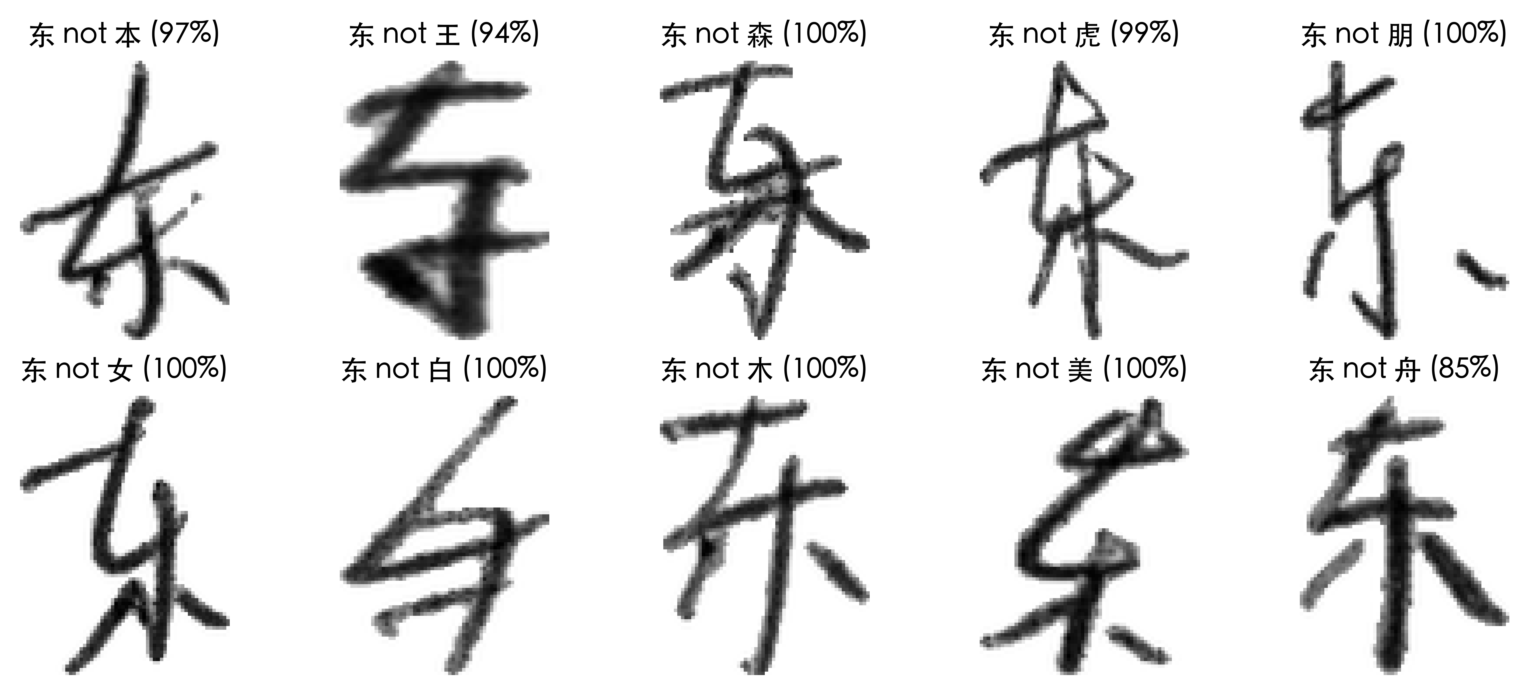
Confidence of predictions
y_log = model.predict(X_test, verbose=0)
y_pred = keras.ops.convert_to_numpy(keras.activations.softmax(y_log))
y_pred_class = np.argmax(y_pred, axis=1)
y_pred_prob = y_pred[np.arange(y_pred.shape[0]), y_pred_class]

confidence_when_correct = y_pred_prob[y_pred_class == y_test]
confidence_when_wrong = y_pred_prob[y_pred_class != y_test]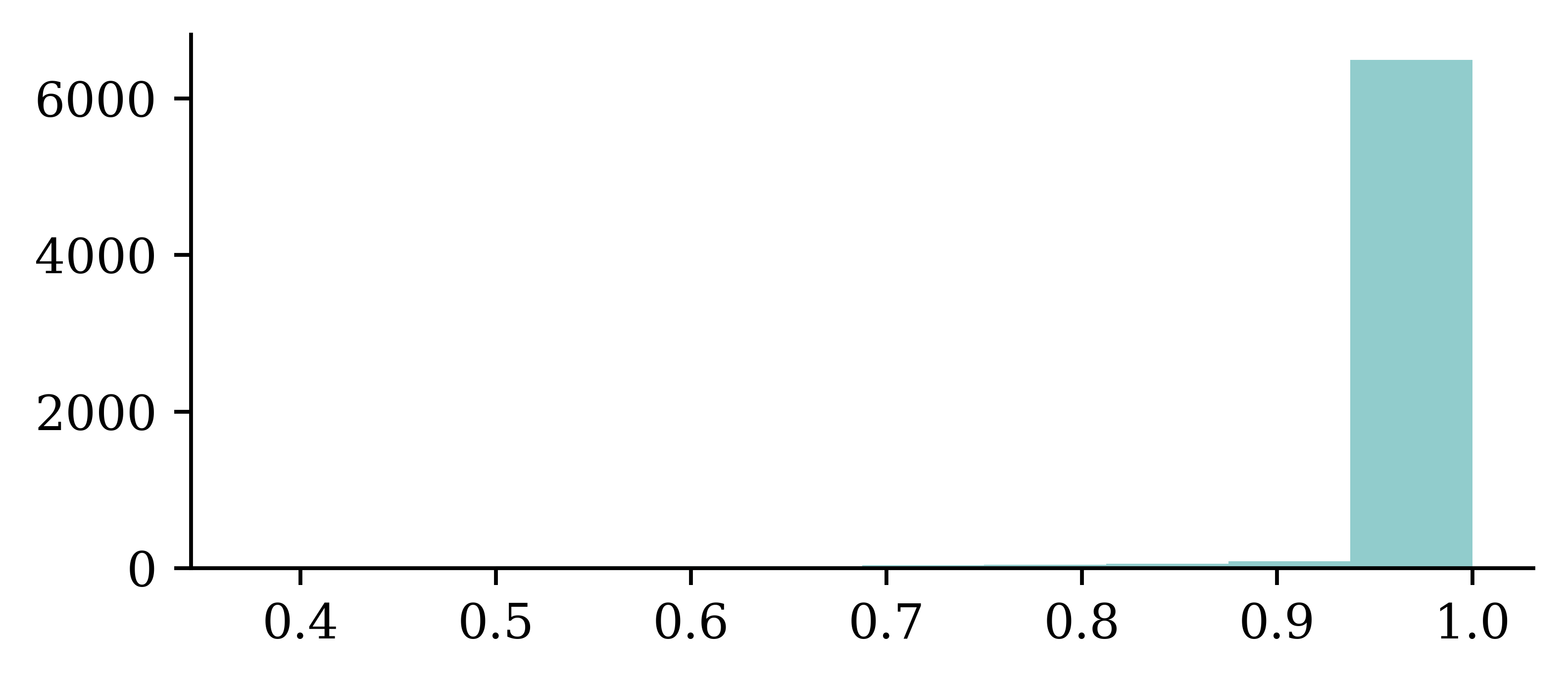
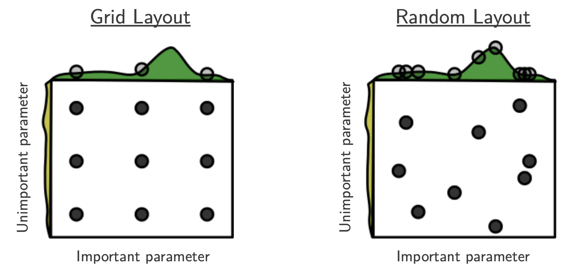
Could we just try every combination?
This technique, called grid search, would be too slow. Better to take random selections.
 .
.
Demo: Object classification

“… these models use a technique called transfer learning. There’s a pretrained neural network, and when you create your own classes, you can sort of picture that your classes are becoming the last layer or step of the neural net. Specifically, both the image and pose models are learning off of pretrained mobilenet models …”
Keras Applications
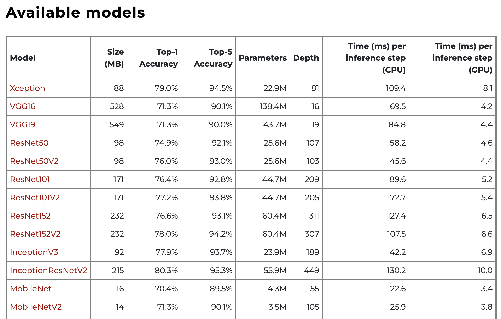
A catalogue of pretrained models at https://keras.io/api/applications/
Each has its own preprocess function that you need to apply to new inputs.
Predicted classes (MobileNet)
Image #0:
 n04399382 - teddy 89%
 n04254120 - soap_dispenser 7%
 n04462240 - toyshop 2%

Image #1:
 n03075370 - combination_lock 30%
 n04019541 - puck 26%
 n03666591 - lighter 10%

Image #2:
 n04009552 - projector 20%
 n03908714 - pencil_sharpener 17%
 n02951585 - can_opener 9%
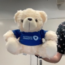

Predicted classes (InceptionV3)
Image #0:
 n04399382 - teddy 87%
 n04162706 - seat_belt 2%
 n04462240 - toyshop 2%

Image #1:
 n04023962 - punching_bag 13%
 n03337140 - file 7%
 n02992529 - cellular_telephone 3%

Image #2:
 n04005630 - prison 4%
 n03337140 - file 4%
 n06596364 - comic_book 2%
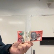
Predicted classes III (MobileNet)
Image #0:
n04350905 - suit 39%
n04591157 - Windsor_tie 34%
n02749479 - assault_rifle 13%
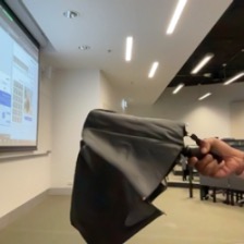
Image #1:
n03529860 - home_theater 25%
n02749479 - assault_rifle 9%
n04009552 - projector 5%
Image #2:
n03529860 - home_theater 9%
n03924679 - photocopier 7%
n02786058 - Band_Aid 6%


Predicted classes III (InceptionV3)
Image #0:
 n04350905 - suit 25%
 n04591157 - Windsor_tie 11%
 n03630383 - lab_coat 6%

Image #1:
 n04507155 - umbrella 52%
 n04404412 - television 2%
 n03529860 - home_theater 2%

Image #2:
 n04404412 - television 17%
 n02777292 - balance_beam 7%
 n03942813 - ping-pong_ball 6%
The original pretrained model
