Classification

ACTL3143 & ACTL5111 Deep Learning for Actuaries

Patrick Laub

Example 1: Binary Classification

Lecture Outline

  • Example 1: Binary Classification

  • Example 2: Multiclass Classification

  • Summary

Stroke Prediction Data description

  1. id: unique identifier
  2. gender: “Male”, “Female” or “Other”
  3. age: age of the patient
  4. hypertension: 0 or 1 if the patient has hypertension
  5. heart_disease: 0 or 1 if the patient has any heart disease
  6. ever_married: “No” or “Yes”
  7. work_type: “children”, “Govt_jov”, “Never_worked”, “Private” or “Self-employed”
  1. Residence_type: “Rural” or “Urban”
  2. avg_glucose_level: average glucose level in blood
  3. bmi: body mass index
  4. smoking_status: “formerly smoked”, “never smoked”, “smokes” or “Unknown”
  5. stroke: 0 or 1 if the patient had a stroke

Load up the (pre-)preprocessed data

PROCESSED_DATA_DIR = Path("stroke/processed")

X_train = pd.read_csv(PROCESSED_DATA_DIR / "x_train.csv")
X_val= pd.read_csv(PROCESSED_DATA_DIR / "x_val.csv")
X_test = pd.read_csv(PROCESSED_DATA_DIR / "x_test.csv")
y_train = pd.read_csv(PROCESSED_DATA_DIR / "y_train.csv")
y_val = pd.read_csv(PROCESSED_DATA_DIR / "y_val.csv")
y_test = pd.read_csv(PROCESSED_DATA_DIR / "y_test.csv")

X_train
gender_Female gender_Male ever_married_No ever_married_Yes Residence_type_Rural Residence_type_Urban work_type_Govt_job work_type_Never_worked work_type_Private work_type_Self-employed work_type_children smoking_status_Unknown smoking_status_formerly smoked smoking_status_never smoked smoking_status_smokes hypertension heart_disease age avg_glucose_level bmi
0 0.0 1.0 0.0 1.0 1.0 0.0 0.0 0.0 1.0 0.0 0.0 0.0 0.0 1.0 0.0 0 0 0.003896 -0.628661 0.005109
1 0.0 1.0 1.0 0.0 1.0 0.0 0.0 0.0 0.0 0.0 1.0 1.0 0.0 0.0 0.0 0 0 -1.634096 -0.257346 -1.509505
2 0.0 1.0 1.0 0.0 1.0 0.0 0.0 0.0 1.0 0.0 0.0 0.0 0.0 1.0 0.0 0 0 -0.483075 -0.754323 -0.732780
... ... ... ... ... ... ... ... ... ... ... ... ... ... ... ... ... ... ... ... ...
3063 1.0 0.0 0.0 1.0 1.0 0.0 1.0 0.0 0.0 0.0 0.0 0.0 0.0 1.0 0.0 1 0 0.667946 -1.028773 0.561761
3064 1.0 0.0 0.0 1.0 1.0 0.0 0.0 0.0 1.0 0.0 0.0 0.0 1.0 0.0 0.0 0 0 -0.084644 -0.366428 0.548816
3065 0.0 1.0 1.0 0.0 0.0 1.0 0.0 0.0 1.0 0.0 0.0 1.0 0.0 0.0 0.0 0 0 -1.147126 -0.765668 -0.422090

3066 rows × 20 columns

Target variable

y_train
stroke
0 0
1 0
2 0
... ...
3063 0
3064 0
3065 0

3066 rows × 1 columns

import numpy as np
classes, counts = np.unique(y_train.values.ravel(), return_counts=True)
print("Classes:", classes)
print("Counts:", counts)
Classes: [0 1]
Counts: [2909  157]

Setup a binary classification model

def create_model(seed=42):
    random.seed(seed)
    model = Sequential()
    model.add(Input(X_train.shape[1:]))
    model.add(Dense(32, "leaky_relu"))
    model.add(Dense(16, "leaky_relu"))
    model.add(Dense(1, "sigmoid"))
    return model
model = create_model()
model.summary()
Model: "sequential"
┏━━━━━━━━━━━━━━━━━━━━━━━━━━━━━━━━━┳━━━━━━━━━━━━━━━━━━━━━━━━┳━━━━━━━━━━━━━━━┓
┃ Layer (type)                     Output Shape                  Param # ┃
┡━━━━━━━━━━━━━━━━━━━━━━━━━━━━━━━━━╇━━━━━━━━━━━━━━━━━━━━━━━━╇━━━━━━━━━━━━━━━┩
│ dense (Dense)                   │ (None, 32)             │           672 │
├─────────────────────────────────┼────────────────────────┼───────────────┤
│ dense_1 (Dense)                 │ (None, 16)             │           528 │
├─────────────────────────────────┼────────────────────────┼───────────────┤
│ dense_2 (Dense)                 │ (None, 1)              │            17 │
└─────────────────────────────────┴────────────────────────┴───────────────┘
 Total params: 1,217 (4.75 KB)
 Trainable params: 1,217 (4.75 KB)
 Non-trainable params: 0 (0.00 B)

Fit the model

model = create_model()
model.compile("adam", "binary_crossentropy")
model.fit(X_train, y_train, epochs=5, verbose=2)
Epoch 1/5
96/96 - 0s - 4ms/step - loss: 0.2732
Epoch 2/5
96/96 - 0s - 617us/step - loss: 0.1701
Epoch 3/5
96/96 - 0s - 619us/step - loss: 0.1632
Epoch 4/5
96/96 - 0s - 626us/step - loss: 0.1603
Epoch 5/5
96/96 - 0s - 629us/step - loss: 0.1587
<keras.src.callbacks.history.History at 0x3063e6a50>

Track accuracy as the model trains

model = create_model()
model.compile("adam", "binary_crossentropy", metrics=["accuracy"])
model.fit(X_train, y_train, epochs=5, verbose=2)
Epoch 1/5
96/96 - 0s - 4ms/step - accuracy: 0.9393 - loss: 0.2732
Epoch 2/5
96/96 - 0s - 659us/step - accuracy: 0.9488 - loss: 0.1701
Epoch 3/5
96/96 - 0s - 661us/step - accuracy: 0.9488 - loss: 0.1632
Epoch 4/5
96/96 - 0s - 653us/step - accuracy: 0.9488 - loss: 0.1603
Epoch 5/5
96/96 - 0s - 658us/step - accuracy: 0.9488 - loss: 0.1587
<keras.src.callbacks.history.History at 0x3063a7cd0>

Run a long fit

model = create_model()
model.compile("adam", "binary_crossentropy", metrics=["accuracy"])
%time hist = model.fit(X_train, y_train, epochs=500, validation_data=(X_val, y_val), verbose=False)
CPU times: user 53 s, sys: 5.54 s, total: 58.5 s
Wall time: 48.3 s

Add early stopping

model = create_model()
model.compile("adam", "binary_crossentropy", metrics=["accuracy"])
es = EarlyStopping(restore_best_weights=True, patience=50, monitor="val_accuracy")
%time hist_es = model.fit(X_train, y_train, epochs=500, validation_data=(X_val, y_val), callbacks=[es], verbose=False)
print(f"Stopped after {len(hist_es.history['loss'])} epochs.")
CPU times: user 5.96 s, sys: 648 ms, total: 6.6 s
Wall time: 5.45 s
Stopped after 51 epochs.

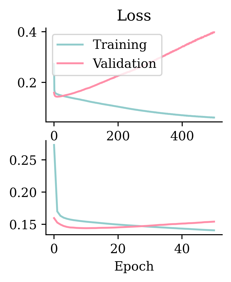
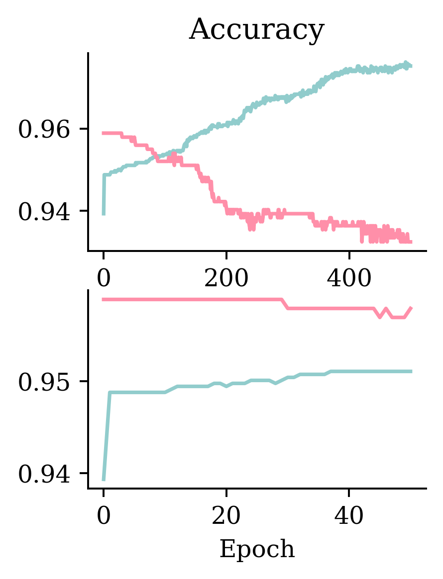
Fitting metrics

Code
matplotlib.pyplot.rcParams["figure.figsize"] = (2.5, 2.95)
plt.subplot(2, 1, 1)
plt.plot(hist.history["loss"])
plt.plot(hist.history["val_loss"])
plt.title("Loss")
plt.legend(["Training", "Validation"])

plt.subplot(2, 1, 2)
plt.plot(hist_es.history["loss"])
plt.plot(hist_es.history["val_loss"])
plt.xlabel("Epoch");

Code
matplotlib.pyplot.rcParams["figure.figsize"] = (2.5, 3.25)
plt.subplot(2, 1, 1)
plt.plot(hist.history["accuracy"])
plt.plot(hist.history["val_accuracy"])
plt.title("Accuracy")

plt.subplot(2, 1, 2)
plt.plot(hist_es.history["accuracy"])
plt.plot(hist_es.history["val_accuracy"])
plt.xlabel("Epoch");

Add metrics, compile, and fit

model = create_model()

pr_auc = keras.metrics.AUC(curve="PR", name="pr_auc")
model.compile(optimizer="adam", loss="binary_crossentropy",
    metrics=[pr_auc, "accuracy", "auc"])                                

es = EarlyStopping(patience=50, restore_best_weights=True,
    monitor="val_pr_auc", verbose=1)
model.fit(X_train, y_train, callbacks=[es], epochs=1_000, verbose=0,
  validation_data=(X_val, y_val));
Epoch 65: early stopping
Restoring model weights from the end of the best epoch: 15.
model.evaluate(X_val, y_val, verbose=0)
[0.14444081485271454,
 0.13122102618217468,
 0.9589040875434875,
 0.8215014934539795]

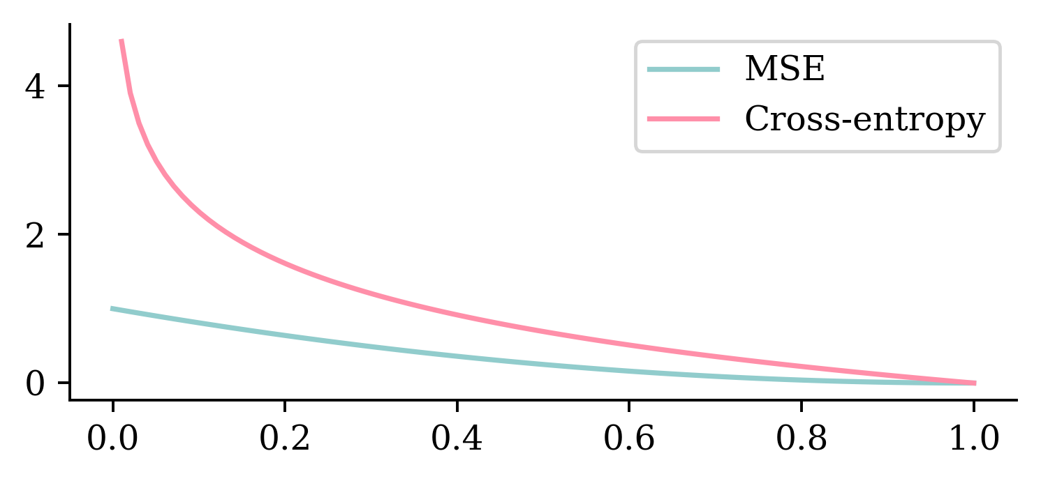
Cross-entropy loss: ELI5

Why use cross-entropy loss?

p = np.linspace(0, 1, 100)
plt.plot(p, (1 - p) ** 2)
plt.plot(p, -np.log(p))
plt.legend(["MSE", "Cross-entropy"]);

Overweight the minority class

model = create_model()

pr_auc = keras.metrics.AUC(curve="PR", name="pr_auc")
model.compile(optimizer="adam", loss="binary_crossentropy",
    metrics=[pr_auc, "accuracy", "auc"])

es = EarlyStopping(patience=50, restore_best_weights=True,
    monitor="val_pr_auc", verbose=1)
model.fit(X_train, y_train.to_numpy(), callbacks=[es], epochs=1_000, verbose=0,
  validation_data=(X_val, y_val), class_weight={0: 1, 1: 10});
Epoch 74: early stopping
Restoring model weights from the end of the best epoch: 24.
model.evaluate(X_val, y_val, verbose=0)
[0.3345569670200348,
 0.13615098595619202,
 0.8062622547149658,
 0.812220573425293]
model.evaluate(X_test, y_test, verbose=0)
[0.3590189516544342, 0.1449822038412094, 0.8023483157157898, 0.791563868522644]

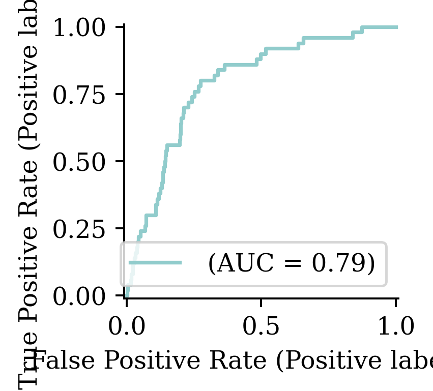
Classification Metrics

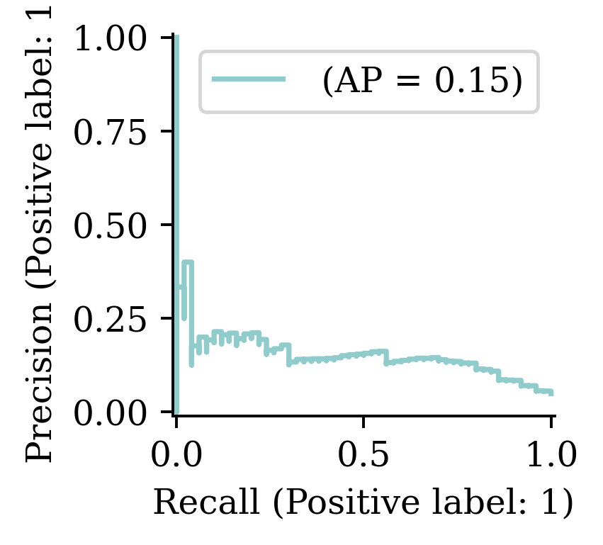
from sklearn.metrics import confusion_matrix, RocCurveDisplay, PrecisionRecallDisplay
y_pred = model.predict(X_test, verbose=0)
RocCurveDisplay.from_predictions(y_test, y_pred, name="");

PrecisionRecallDisplay.from_predictions(y_test, y_pred, name=""); plt.legend(loc="upper right");

y_pred_stroke = y_pred > 0.5
confusion_matrix(y_test, y_pred_stroke)
array([[792, 180],
       [ 22,  28]])
y_pred_stroke = y_pred > 0.3
confusion_matrix(y_test, y_pred_stroke)
array([[662, 310],
       [ 10,  40]])

Example 2: Multiclass Classification

Lecture Outline

  • Example 1: Binary Classification

  • Example 2: Multiclass Classification

  • Summary

Iris dataset

from sklearn.datasets import load_iris
iris = load_iris()
names = ["SepalLength", "SepalWidth", "PetalLength", "PetalWidth"]
features = pd.DataFrame(iris.data, columns=names)
features
SepalLength SepalWidth PetalLength PetalWidth
0 5.1 3.5 1.4 0.2
1 4.9 3.0 1.4 0.2
... ... ... ... ...
148 6.2 3.4 5.4 2.3
149 5.9 3.0 5.1 1.8

150 rows × 4 columns

Target variable

iris.target_names
array(['setosa', 'versicolor', 'virginica'], dtype='<U10')
iris.target[:8]
array([0, 0, 0, 0, 0, 0, 0, 0])
target = iris.target
target = target.reshape(-1, 1)
target[:8]
array([[0],
       [0],
       [0],
       [0],
       [0],
       [0],
       [0],
       [0]])
classes, counts = np.unique(
        target,
        return_counts=True
)
print(classes)
print(counts)
[0 1 2]
[50 50 50]
iris.target_names[
  target[[0, 30, 60]]
]
array([['setosa'],
       ['setosa'],
       ['versicolor']], dtype='<U10')

Split the data into train and test

X_train, X_test, y_train, y_test = train_test_split(features, target, random_state=24)
X_train
SepalLength SepalWidth PetalLength PetalWidth
53 5.5 2.3 4.0 1.3
58 6.6 2.9 4.6 1.3
95 5.7 3.0 4.2 1.2
... ... ... ... ...
145 6.7 3.0 5.2 2.3
87 6.3 2.3 4.4 1.3
131 7.9 3.8 6.4 2.0

112 rows × 4 columns

X_test.shape, y_test.shape
((38, 4), (38, 1))

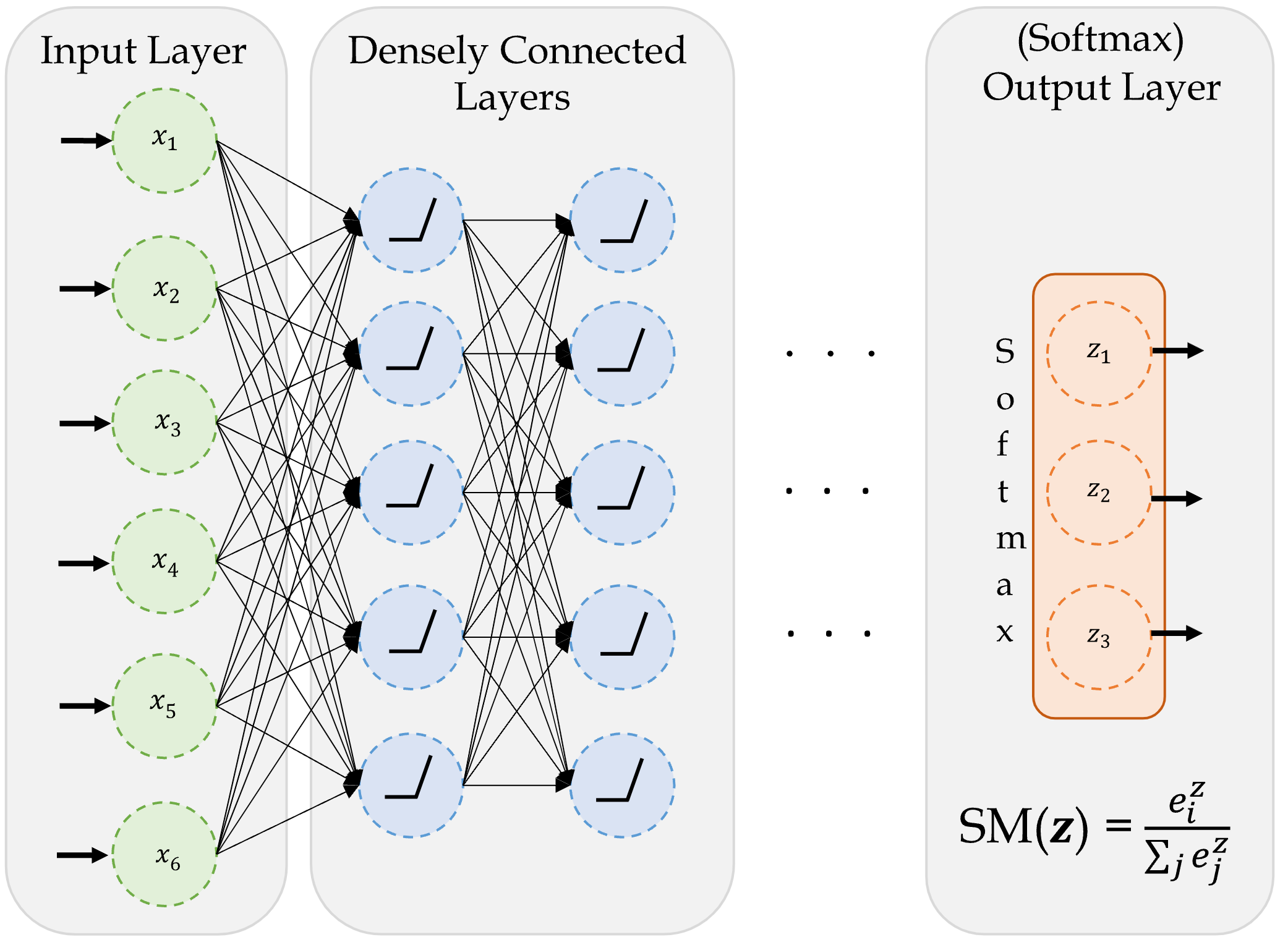
A basic classifier network

A basic network for classifying into three categories.

Create a classifier model

NUM_FEATURES = len(features.columns)
NUM_CATS = len(np.unique(target))

print("Number of features:", NUM_FEATURES)
print("Number of categories:", NUM_CATS)
Number of features: 4
Number of categories: 3

Make a function to return a Keras model:

def build_model(seed=42):
    random.seed(seed)
    return Sequential([
        Dense(30, activation="relu"),
        Dense(NUM_CATS, activation="softmax")
    ])

Fit the model

model = build_model()
model.compile("adam", "sparse_categorical_crossentropy")

model.fit(X_train, y_train, epochs=5, verbose=2);
Epoch 1/5
4/4 - 0s - 68ms/step - loss: 1.3502
Epoch 2/5
4/4 - 0s - 5ms/step - loss: 1.2852
Epoch 3/5
4/4 - 0s - 5ms/step - loss: 1.2337
Epoch 4/5
4/4 - 0s - 6ms/step - loss: 1.1915
Epoch 5/5
4/4 - 0s - 5ms/step - loss: 1.1556

Track accuracy as the model trains

model = build_model()
model.compile("adam", "sparse_categorical_crossentropy", metrics=["accuracy"])
model.fit(X_train, y_train, epochs=5, verbose=2);
Epoch 1/5
4/4 - 0s - 77ms/step - accuracy: 0.2946 - loss: 1.3502
Epoch 2/5
4/4 - 0s - 6ms/step - accuracy: 0.3036 - loss: 1.2852
Epoch 3/5
4/4 - 0s - 6ms/step - accuracy: 0.3036 - loss: 1.2337
Epoch 4/5
4/4 - 0s - 6ms/step - accuracy: 0.3304 - loss: 1.1915
Epoch 5/5
4/4 - 0s - 5ms/step - accuracy: 0.3393 - loss: 1.1556

Run a long fit

model = build_model()
model.compile("adam", "sparse_categorical_crossentropy", \
        metrics=["accuracy"])
%time hist = model.fit(X_train, y_train, epochs=500, \
        validation_split=0.25, verbose=False)
CPU times: user 19.8 s, sys: 1.74 s, total: 21.6 s
Wall time: 19.9 s

Evaluation now returns both loss and accuracy.

model.evaluate(X_test, y_test, verbose=False)
[0.09586217254400253, 0.9736841917037964]

Add early stopping

model_es = build_model()
model_es.compile("adam", "sparse_categorical_crossentropy", \
        metrics=["accuracy"])

es = EarlyStopping(restore_best_weights=True, patience=50,
        monitor="val_accuracy")                                         
%time hist_es = model_es.fit(X_train, y_train, epochs=500, \
        validation_split=0.25, callbacks=[es], verbose=False);

print(f"Stopped after {len(hist_es.history['loss'])} epochs.")
CPU times: user 2.97 s, sys: 275 ms, total: 3.25 s
Wall time: 2.97 s
Stopped after 68 epochs.

Evaluation on test set:

model_es.evaluate(X_test, y_test, verbose=False)
[0.9856259226799011, 0.5263158082962036]

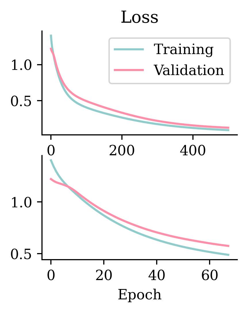
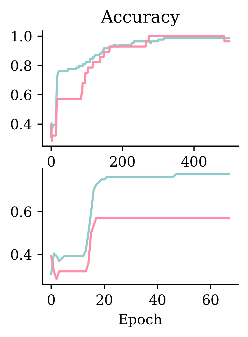
Fitting metrics

Code
matplotlib.pyplot.rcParams["figure.figsize"] = (2.5, 2.95)
plt.subplot(2, 1, 1)
plt.plot(hist.history["loss"])
plt.plot(hist.history["val_loss"])
plt.title("Loss")
plt.legend(["Training", "Validation"])

plt.subplot(2, 1, 2)
plt.plot(hist_es.history["loss"])
plt.plot(hist_es.history["val_loss"])
plt.xlabel("Epoch");

Code
matplotlib.pyplot.rcParams["figure.figsize"] = (2.5, 3.25)
plt.subplot(2, 1, 1)
plt.plot(hist.history["accuracy"])
plt.plot(hist.history["val_accuracy"])
plt.title("Accuracy")

plt.subplot(2, 1, 2)
plt.plot(hist_es.history["accuracy"])
plt.plot(hist_es.history["val_accuracy"])
plt.xlabel("Epoch");

What is the softmax activation?

It creates a “probability” vector: \text{Softmax}(\boldsymbol{x}) = \frac{\mathrm{e}^x_i}{\sum_j \mathrm{e}^x_j} \,.

In NumPy:

out = np.array([5, -1, 6])
(np.exp(out) / np.exp(out).sum()).round(3)
array([0.269, 0.001, 0.731])

In Keras:

out = keras.ops.convert_to_tensor([[5.0, -1.0, 6.0]])
keras.ops.round(keras.ops.softmax(out), 3)
<tf.Tensor: shape=(1, 3), dtype=float32, numpy=array([[0.269, 0.001, 0.731]], dtype=float32)>

Prediction using classifiers

y_test[:4]
array([[2],
       [2],
       [1],
       [1]])
y_pred = model.predict(X_test.head(4), verbose=0)
y_pred
array([[4.9469954e-06, 8.1675522e-02, 9.1831952e-01],
       [4.1672743e-06, 7.0206067e-03, 9.9297523e-01],
       [9.2273308e-03, 9.7335482e-01, 1.7417978e-02],
       [3.1080188e-03, 8.7022400e-01, 1.2666793e-01]], dtype=float32)
# Add 'keepdims=True' to get a column vector.
np.argmax(y_pred, axis=1)
array([2, 2, 1, 1])
iris.target_names[np.argmax(y_pred, axis=1)]
array(['virginica', 'virginica', 'versicolor', 'versicolor'], dtype='<U10')

Summary

Lecture Outline

  • Example 1: Binary Classification

  • Example 2: Multiclass Classification

  • Summary

Classification models in Keras

If the number of classes is c, then:

Target Output Layer Loss Function
Binary
(c=2)
1 neuron with sigmoid activation Binary Cross-Entropy
Multi-class
(c > 2)
c neurons with softmax activation Categorical Cross-Entropy

Optionally output logits

If the number of classes is c, then:

Target Output Layer Loss Function
Binary
(c=2)
1 neuron with linear activation Binary Cross-Entropy (from_logits=True)
Multi-class
(c > 2)
c neurons with linear activation Categorical Cross-Entropy (from_logits=True)

Code examples

Binary

model = Sequential([
  # Skipping the earlier layers
  Dense(1, activation="sigmoid")
])
model.compile(loss="binary_crossentropy")

Multi-class

model = Sequential([
  # Skipping the earlier layers
  Dense(n_classes, activation="softmax")
])
model.compile(loss="sparse_categorical_crossentropy")

Binary (logits)

from keras.losses import BinaryCrossentropy
model = Sequential([
  # Skipping the earlier layers
  Dense(1, activation="linear")
])
loss = BinaryCrossentropy(from_logits=True)
model.compile(loss=loss)

Multi-class (logits)

from keras.losses import SparseCategoricalCrossentropy

model = Sequential([
  # Skipping the earlier layers
  Dense(n_classes, activation="linear")
])
loss = SparseCategoricalCrossentropy(from_logits=True)
model.compile(loss=loss)

Package Versions

from watermark import watermark
print(watermark(python=True, packages="keras,matplotlib,numpy,pandas,seaborn,scipy,torch,tensorflow,tf_keras"))
Python implementation: CPython
Python version       : 3.11.12
IPython version      : 9.3.0

keras     : 3.8.0
matplotlib: 3.10.0
numpy     : 2.0.2
pandas    : 2.2.2
seaborn   : 0.13.2
scipy     : 1.15.3
torch     : 2.6.0
tensorflow: 2.18.0
tf_keras  : 2.18.0

Glossary

  • accuracy
  • classification problem
  • confusion matrix
  • cross-entropy loss
  • metrics
  • sigmoid activation function
  • softmax activation