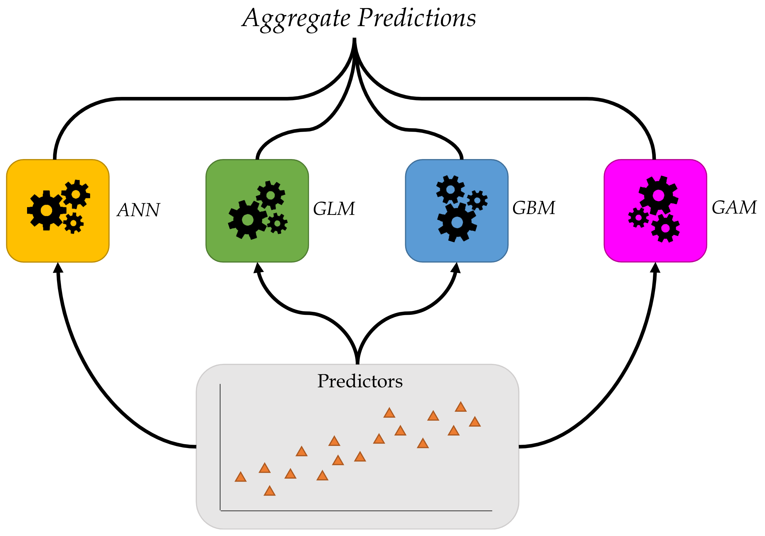
Distributional Regression

ACTL3143 & ACTL5111 Deep Learning for Actuaries

Patrick Laub

Introduction

Lecture Outline

  • Introduction

  • Traditional Regression

  • Stochastic Forecasts

  • GLMs and Neural Networks

  • Combined Actuarial Neural Network

  • Mean-Variance Estimation Network

  • Mixture Density Network

  • Distributional Refinement Network

  • Uncertainty and Regularisation

  • Dropout and Ensembles

Why actuaries avoid neural networks

They’re not inherently interpretable, so we just have to look at inputs and outputs from the black box.

Neural network models typically just output a prediction without any sense of its confidence.

Therefore we cannot trust the neural network models, which is a dealbreaker.

Now let’s focus on actuarial problems.

Car insurance

Claim size prediction

πŸ‘€ Age πŸš— Age 🏎️ Type
25 3 πŸš™ Sedan
40 5 🚐 SUV
19 1 🏎️ Sports Car
60 10 🚘 Hatchback


\longrightarrow

Cost
πŸ’΅ $1,200
πŸ’΅ $2,500
πŸ’΅ $3,800
πŸ’΅ $800

What’s wrong? Not enough rows? Not enough columns?

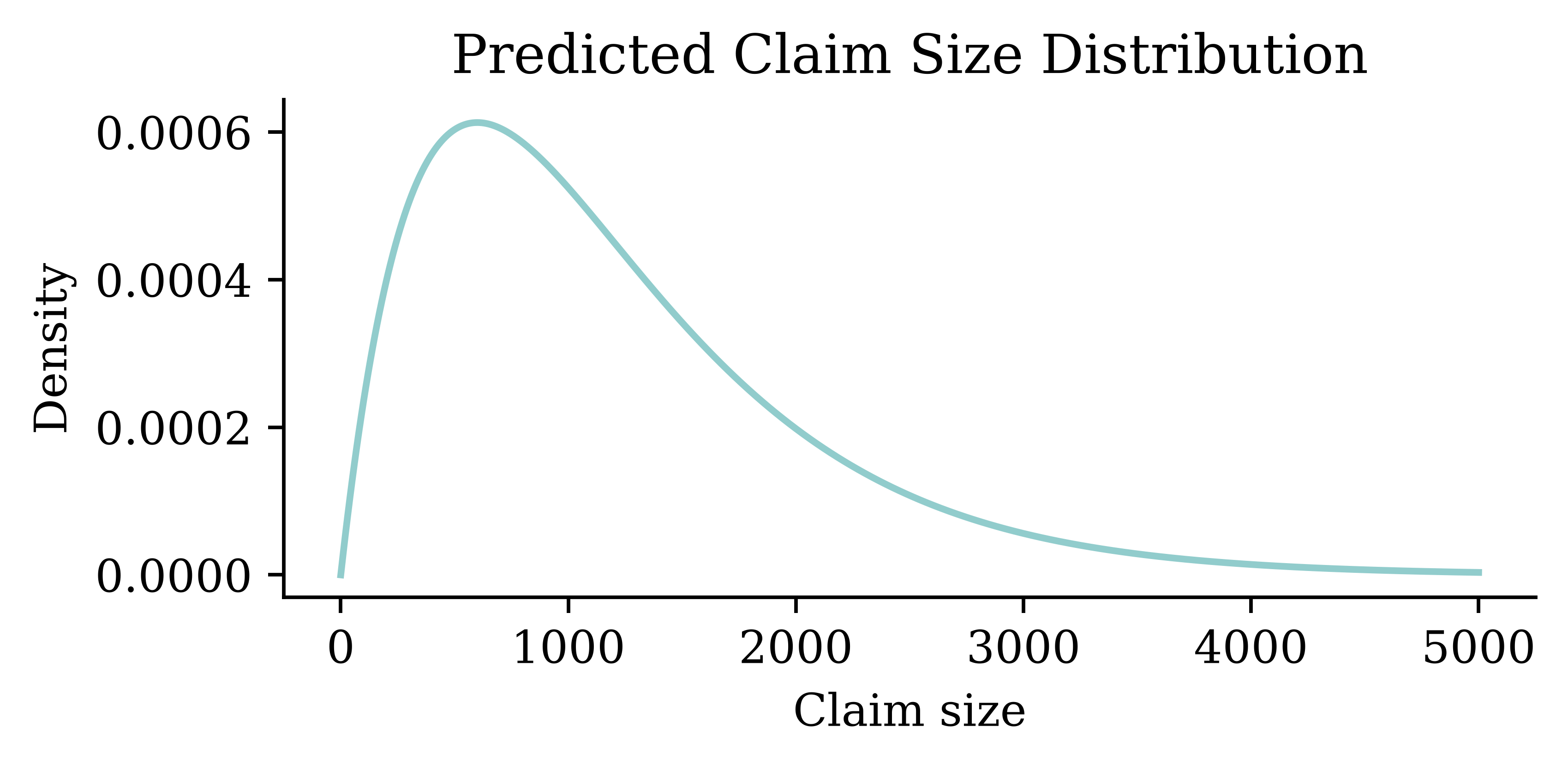
Distributional regression

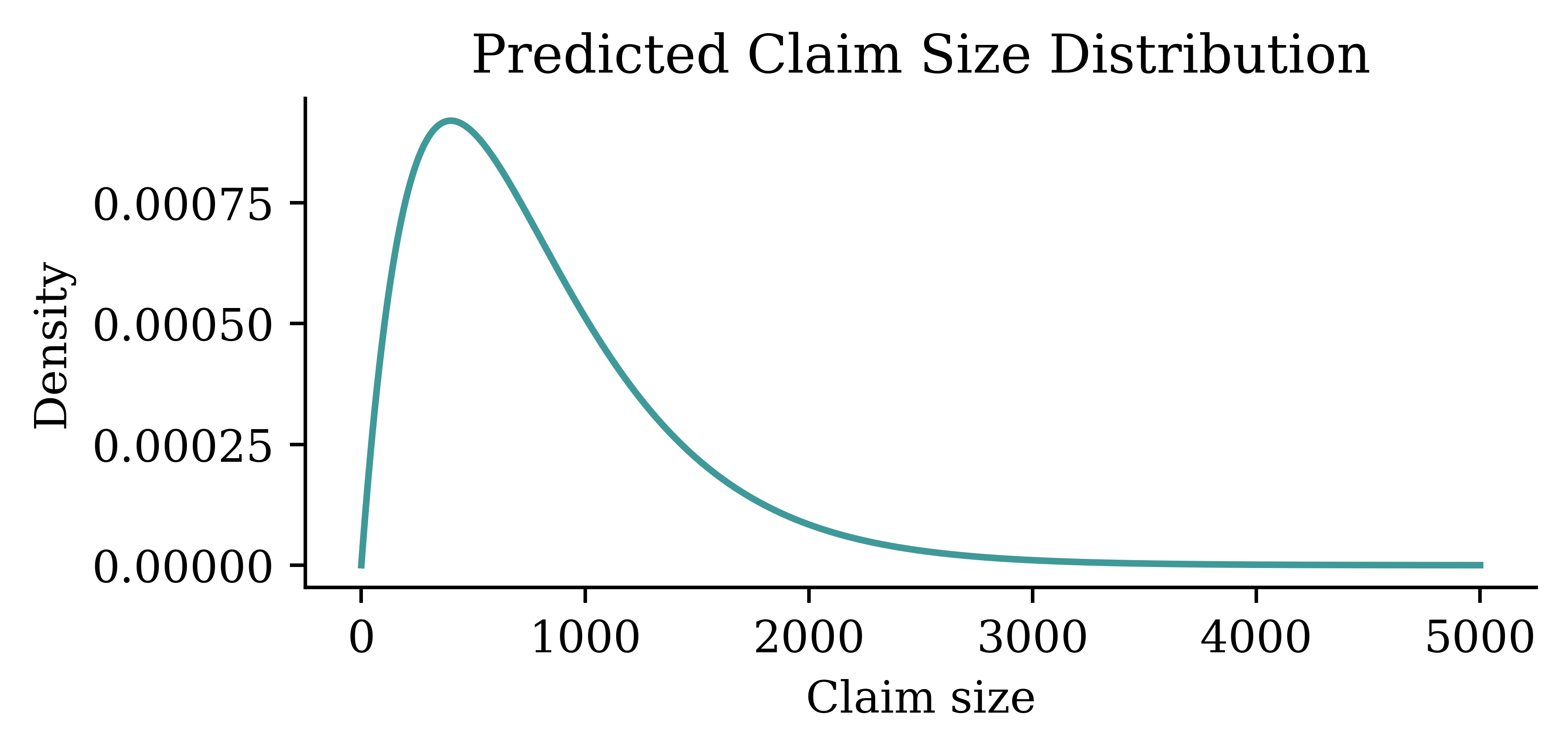
Customer 1 = (25, 3, πŸš™)

Distributional regression

Customer 2 = (40, 5, 🚐)
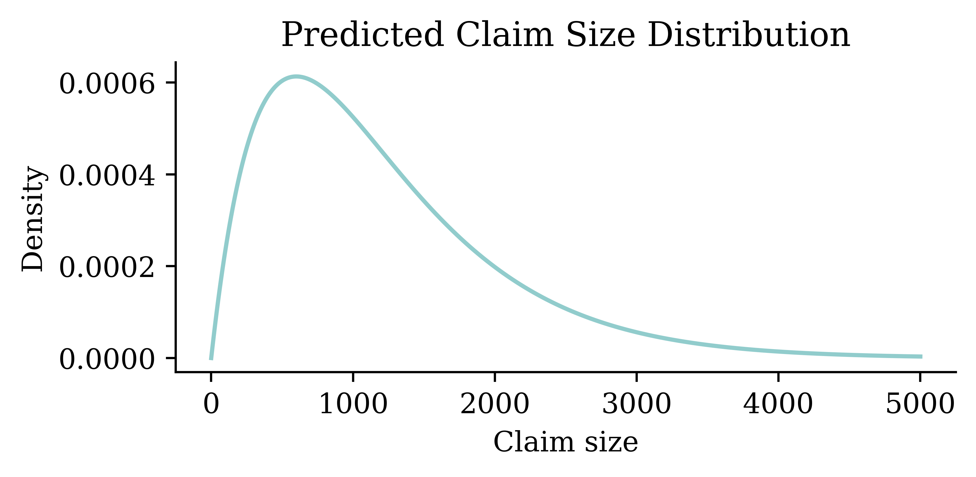
Distributional regression

Customer 3 = (19, 1, 🏎️)
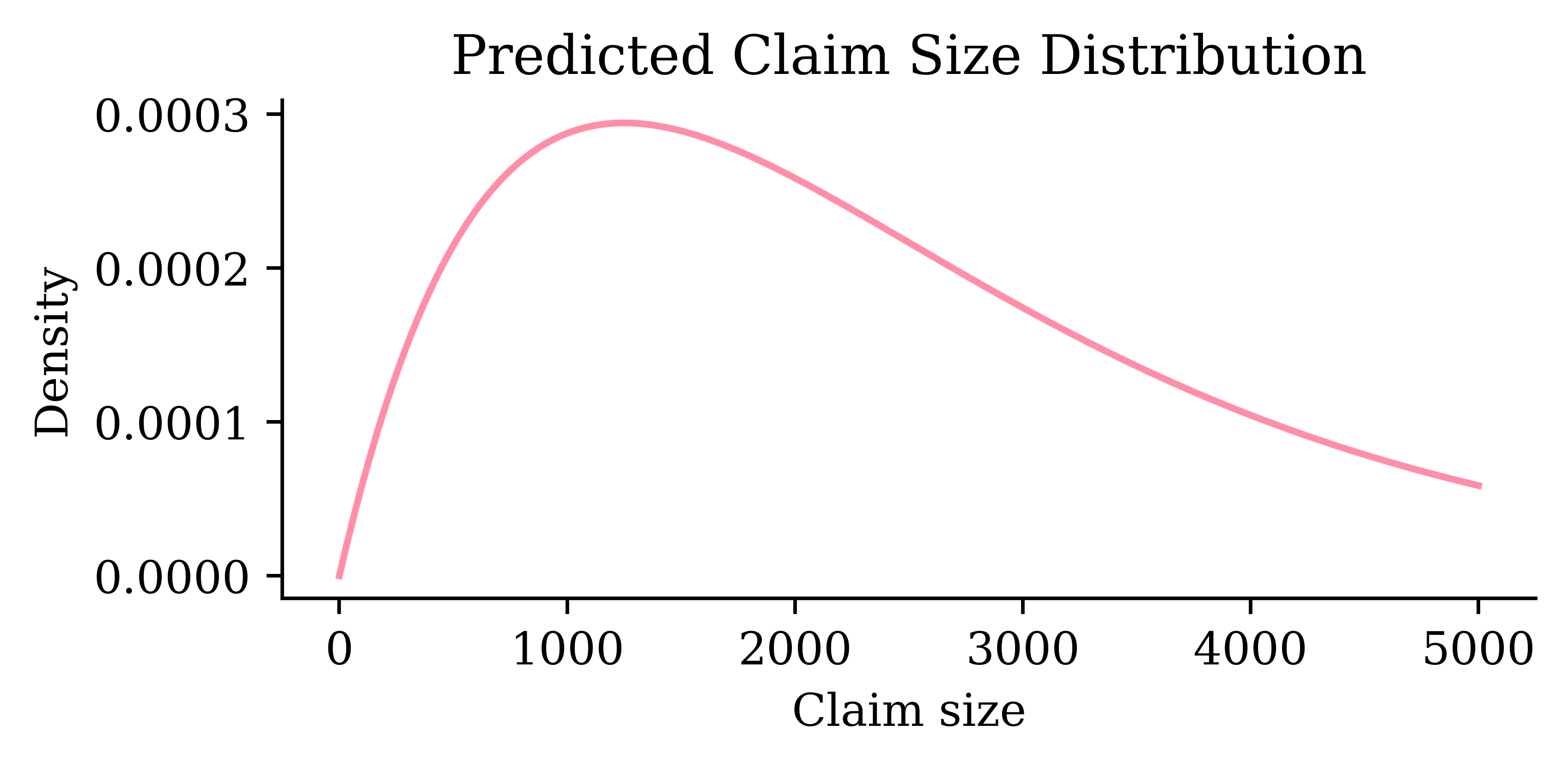
Distributional regression

Customer 4 = (60, 10, 🚘)
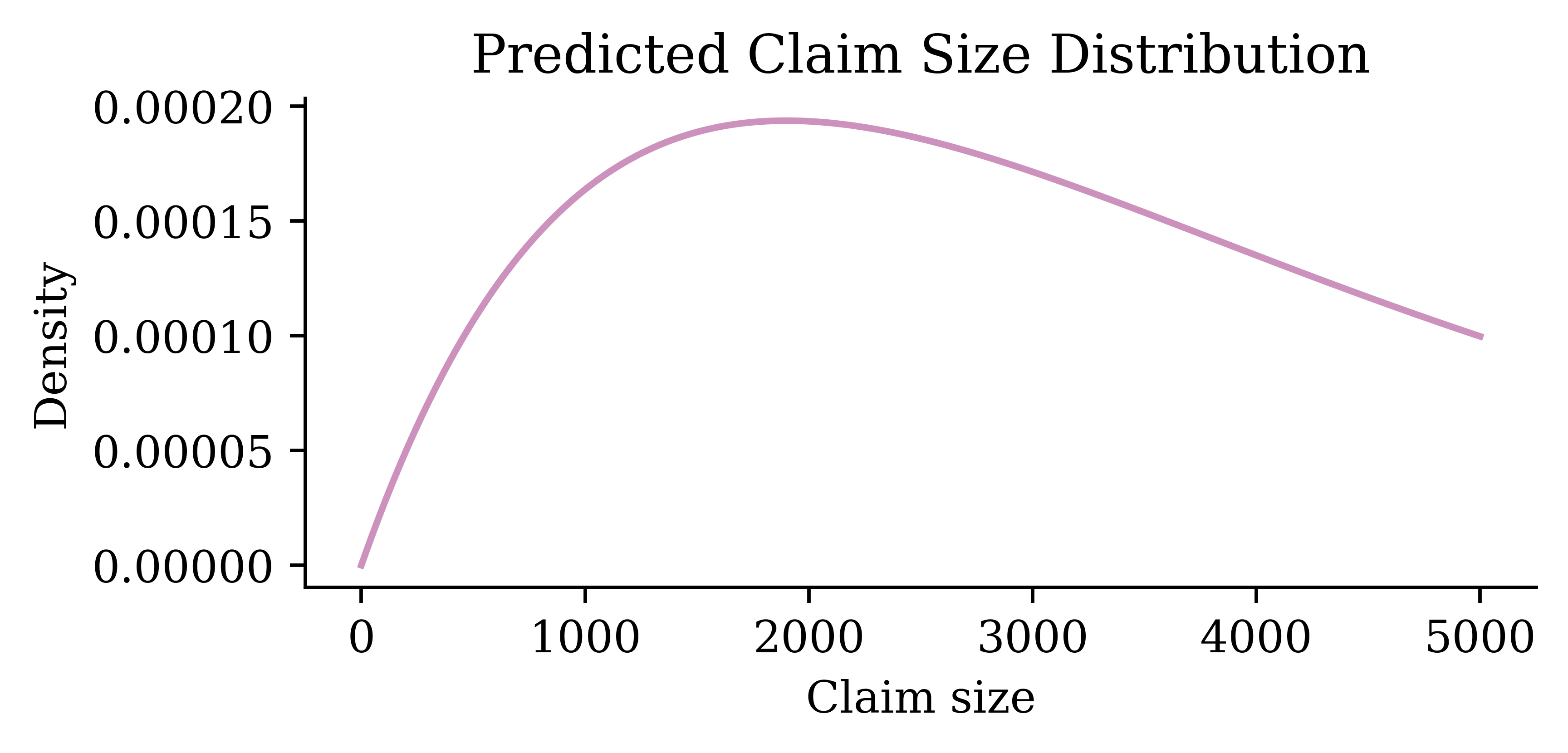
Distributional regression

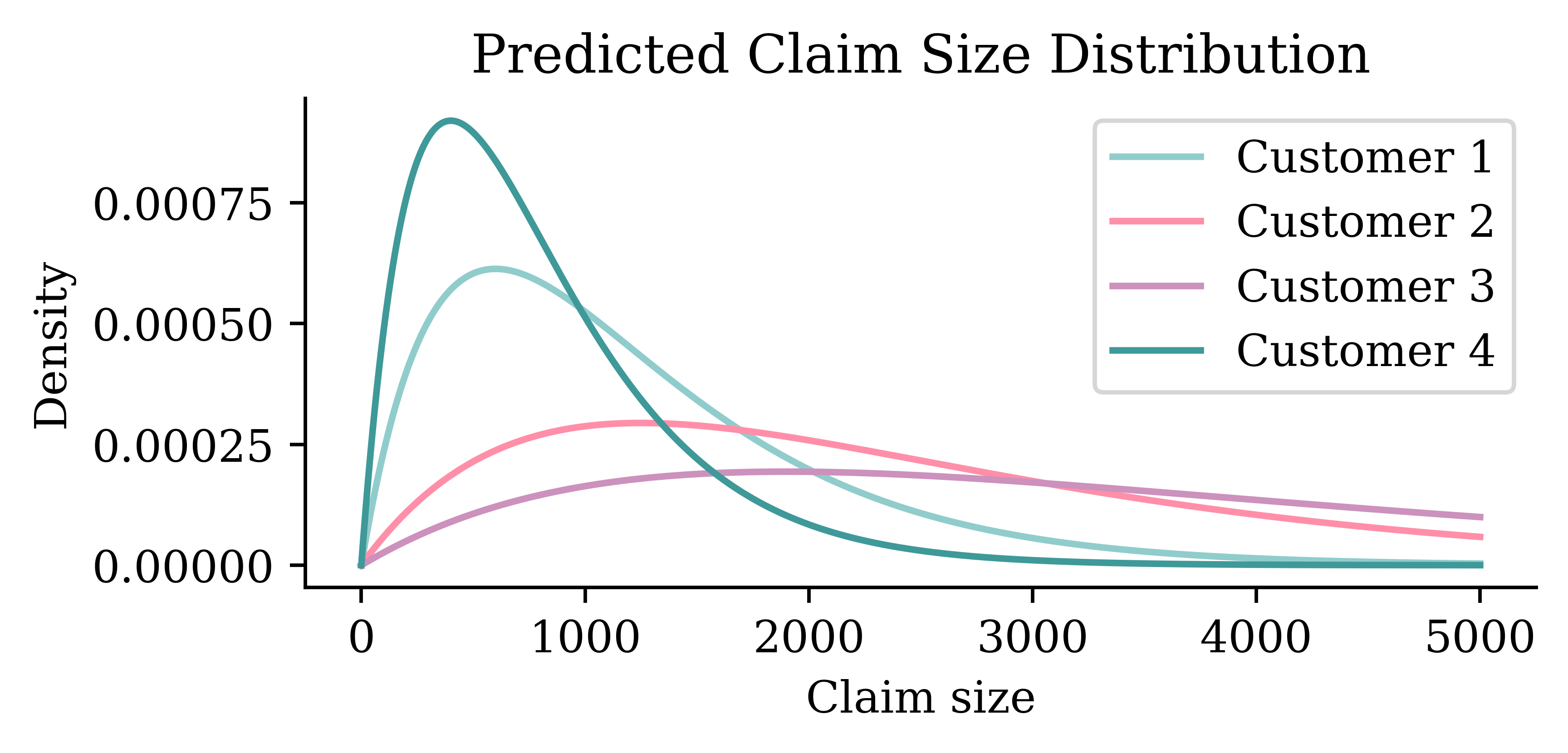
All customers
One model, many distributions

Feed in a batch of customers and the model returns a predicted claim-size distribution for each one.
Predicting distribution parameters

In practice the network doesn’t emit a whole curve β€” it emits the parameters of a chosen distribution family, which then define the distribution.
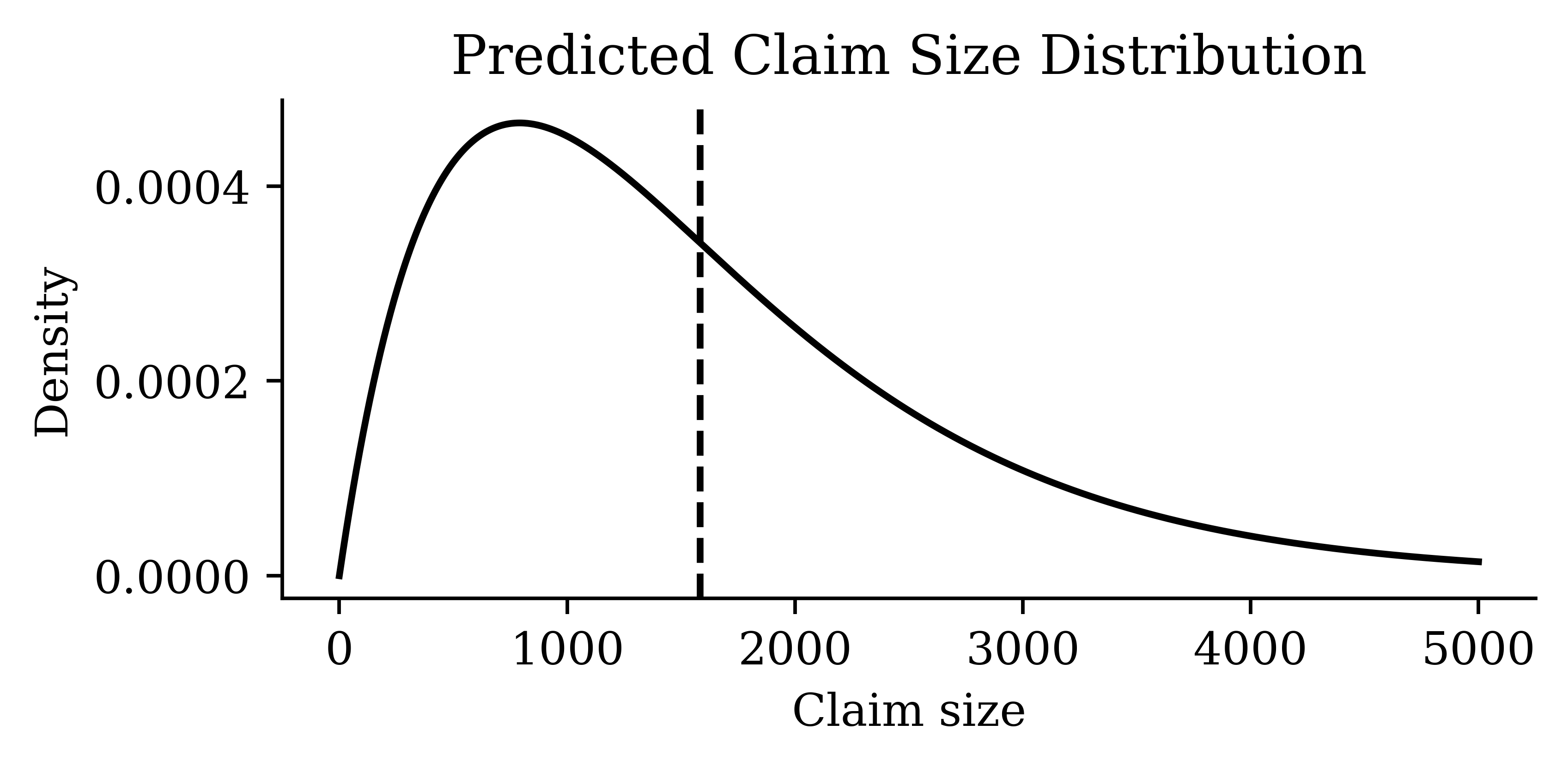
Anatomy of a predicted distribution

From a single predicted distribution we can read off the mean, the variance, and high quantiles (e.g. Value-at-Risk).
Traditional vs distributional regression

Same inputs, same model β€” the difference is what comes out.

Baseline: a generalised linear model

A gamma GLM with a log link function:

\begin{aligned} Y | \mathbf{X} &\sim \mathrm{Gamma}(\ldots, \ldots) \\ \mathbb{E}[Y | \mathbf{X}] &= \exp\Bigl\{ \beta_0 + \beta_1 \cdot \text{Age} + \beta_2 \cdot \text{Car Age} + \beta_3 \cdot \text{Type} \Bigr\} \end{aligned}

A simple model, easy to train and interpret, but…

GLMs can be

  1. Bad at regression
  2. Bad at distributional regression

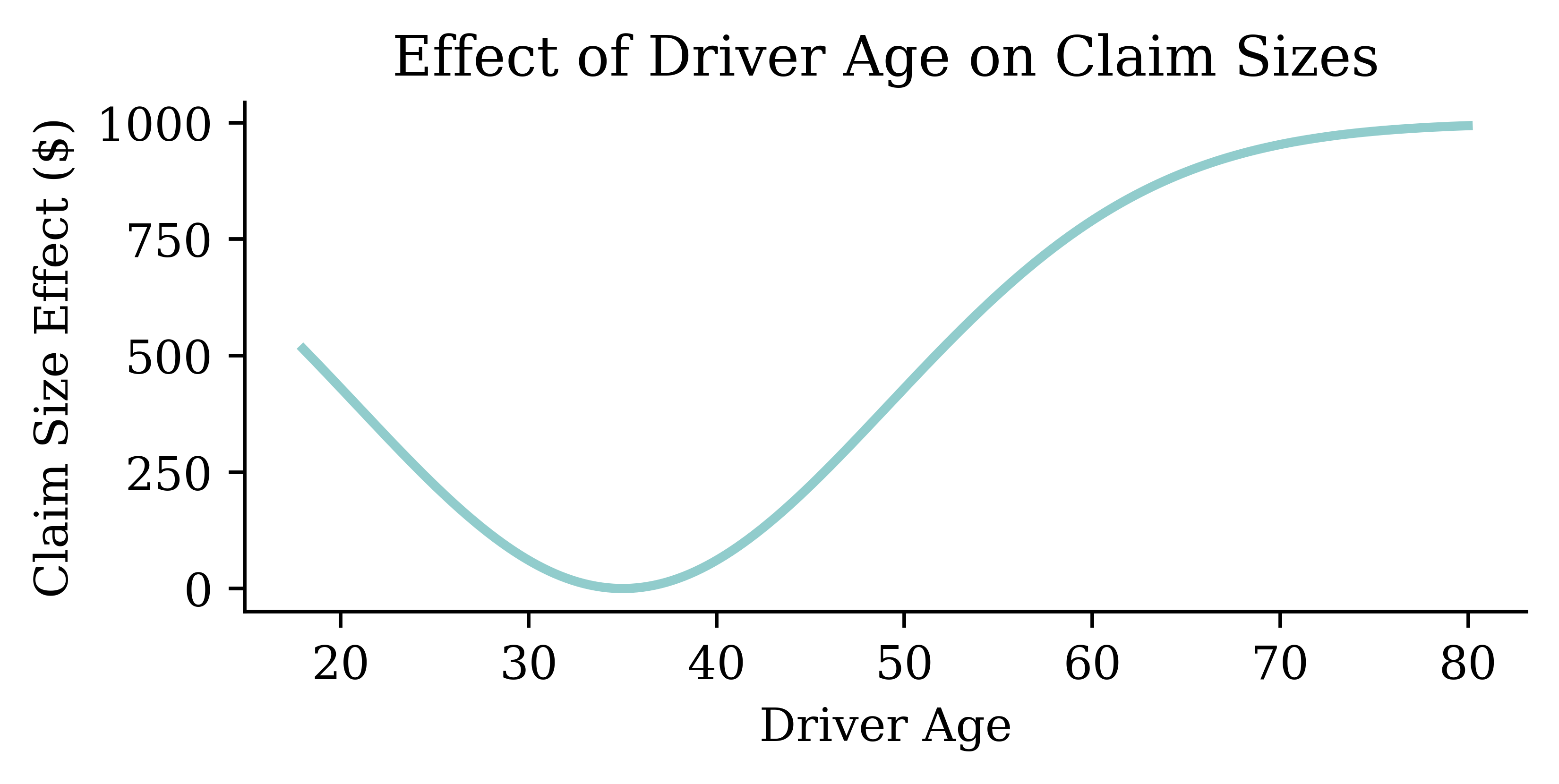
Example 1: Non-monotonicity

GLMs cannot (easily) do this \longrightarrow Use a neural network

Example 2: Multimodality
Key idea
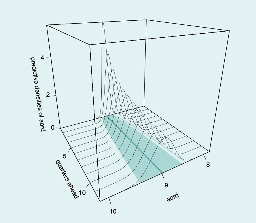
An example of distributional forecasting over the All Ordinaries Index
  • Earlier machine learning models focused on point estimates.
  • However, in many applications, we need to understand the distribution of the response variable.
  • Each prediction becomes a distribution over the possible outcomes

We will focus on regression not classification

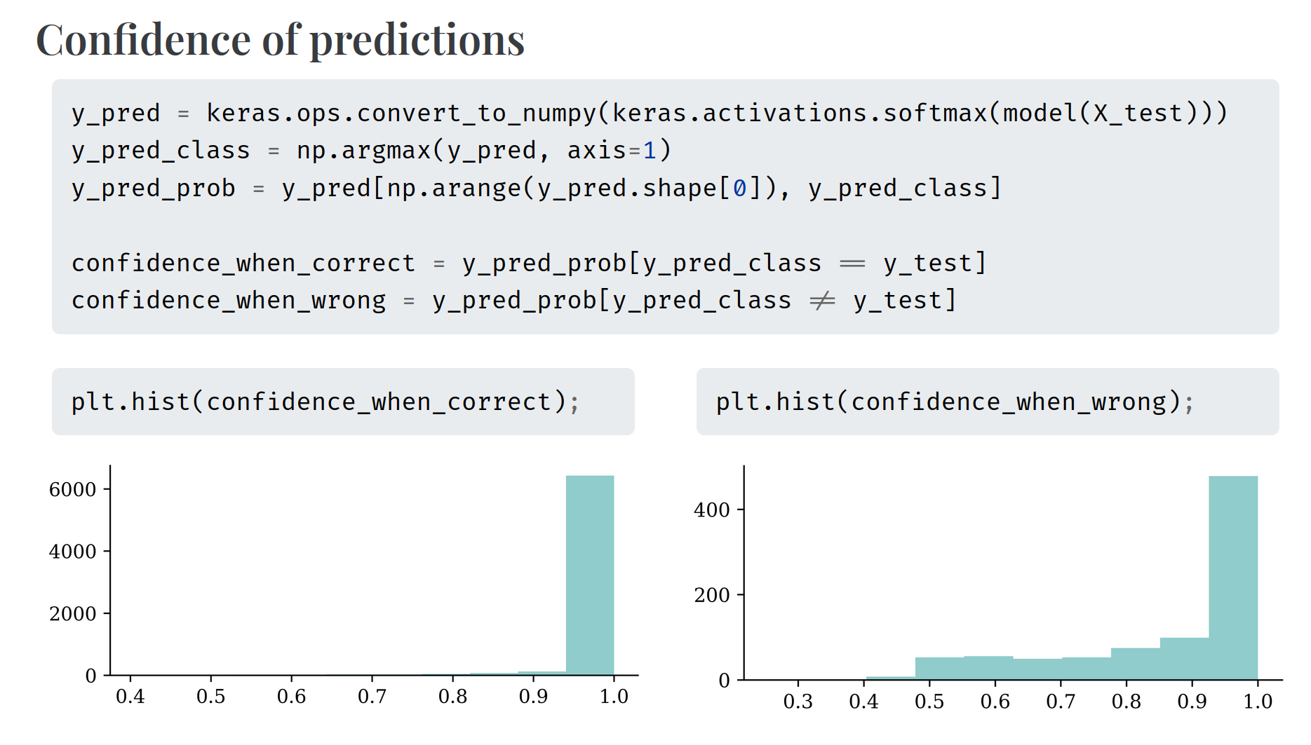
Classifiers already give us a probability, which is a big step up compared to regression models.

However, neural networks’ β€œprobabilities” can be overconfident.

We already saw a case of this.

See Guo et al. (2017).

Traditional Regression

Lecture Outline

  • Introduction

  • Traditional Regression

  • Stochastic Forecasts

  • GLMs and Neural Networks

  • Combined Actuarial Neural Network

  • Mean-Variance Estimation Network

  • Mixture Density Network

  • Distributional Refinement Network

  • Uncertainty and Regularisation

  • Dropout and Ensembles

Package imports

import random
import matplotlib.pyplot as plt
import numpy as np
import pandas as pd

import keras
from keras.models import Sequential, Model
from keras.layers import Input, Dense, Concatenate, Dropout
from keras.callbacks import EarlyStopping
from keras.initializers import Constant
from keras.regularizers import L1, L2

from sklearn.model_selection import train_test_split
from sklearn.compose import make_column_transformer
from sklearn.pipeline import make_pipeline
from sklearn.preprocessing import StandardScaler, OrdinalEncoder
from sklearn.linear_model import LinearRegression
from sklearn.datasets import fetch_california_housing
from sklearn import set_config
set_config(transform_output="pandas")

import scipy.stats as stats
import statsmodels.api as sm
from torch.distributions import Gamma, MixtureSameFamily, Categorical

Notation

  • scalars are denoted by lowercase letters, e.g., y,
  • vectors are denoted by bold lowercase letters, e.g., \boldsymbol{y} = (y_1, \ldots, y_n) ,
  • random variables are denoted by capital letters, e.g., Y
  • random vectors are denoted by bold capital letters, e.g., \boldsymbol{X} = (X_1, \ldots, X_p) ,
  • matrices are denoted by bold uppercase non-italics letters, e.g., \mathbf{X} = \begin{pmatrix} x_{11} & \cdots & x_{1p} \\ \vdots & \ddots & \vdots \\ x_{n1} & \cdots & x_{np} \end{pmatrix} .

Regression notation

  • n is the number of observations, p is the number of features,
  • the true coefficients are \boldsymbol{\beta} = (\beta_0, \beta_1, \ldots, \beta_p),
  • \beta_0 is the intercept, \beta_1, \ldots, \beta_p are the coefficients,
  • \boldsymbol{\beta}^* is the estimated coefficient vector,
  • \boldsymbol{x}_i = (1, x_{i1}, x_{i2}, \ldots, x_{ip}) is the feature vector for the ith observation,
  • y_i is the response variable for the ith observation,
  • \hat{y}_i is the predicted value for the ith observation,

Distributional assumptions become loss functions

Each example below follows the same maximum-likelihood recipe:

  1. Choose a distribution and write its density or mass function.

    Y_i|\boldsymbol{X}=\boldsymbol{x}_i \sim F(\theta_i), \qquad f(y_i; \theta_i)

  2. Multiply the probabilities to form the likelihood.

    L(\boldsymbol{\beta}) = \prod_{i=1}^n f(y_i; \theta_i)

  3. Take logs to get the log-likelihood and negate it to get negative log likelihood.

    \ell(\boldsymbol{\beta}) = \sum_{i=1}^n \log f(y_i; \theta_i) \quad \Rightarrow \text{NLL}(\boldsymbol{\beta}) = -\ell(\boldsymbol{\beta})

  4. Drop constants and rescale to get the model loss.

    \text{loss}(\boldsymbol{y}, \hat{\boldsymbol{y}})

Traditional regression

Multiple linear regression assumes the data-generating process is

Y_i = \beta_0 + \beta_1 x_{i1} + \beta_2 x_{i2} + \ldots + \beta_p x_{ip} + \varepsilon

where \varepsilon \sim \mathcal{N}(0, \sigma^2).

We estimate the coefficients \beta_0, \beta_1, \ldots, \beta_p by minimising the sum of squared residuals or mean squared error

\text{RSS} := \sum_{i=1}^n (y_i - \hat{y}_i)^2 , \quad \text{MSE} := \frac{1}{n} \sum_{i=1}^n (y_i - \hat{y}_i)^2 ,

where \hat{y}_i is the predicted value for the ith observation.

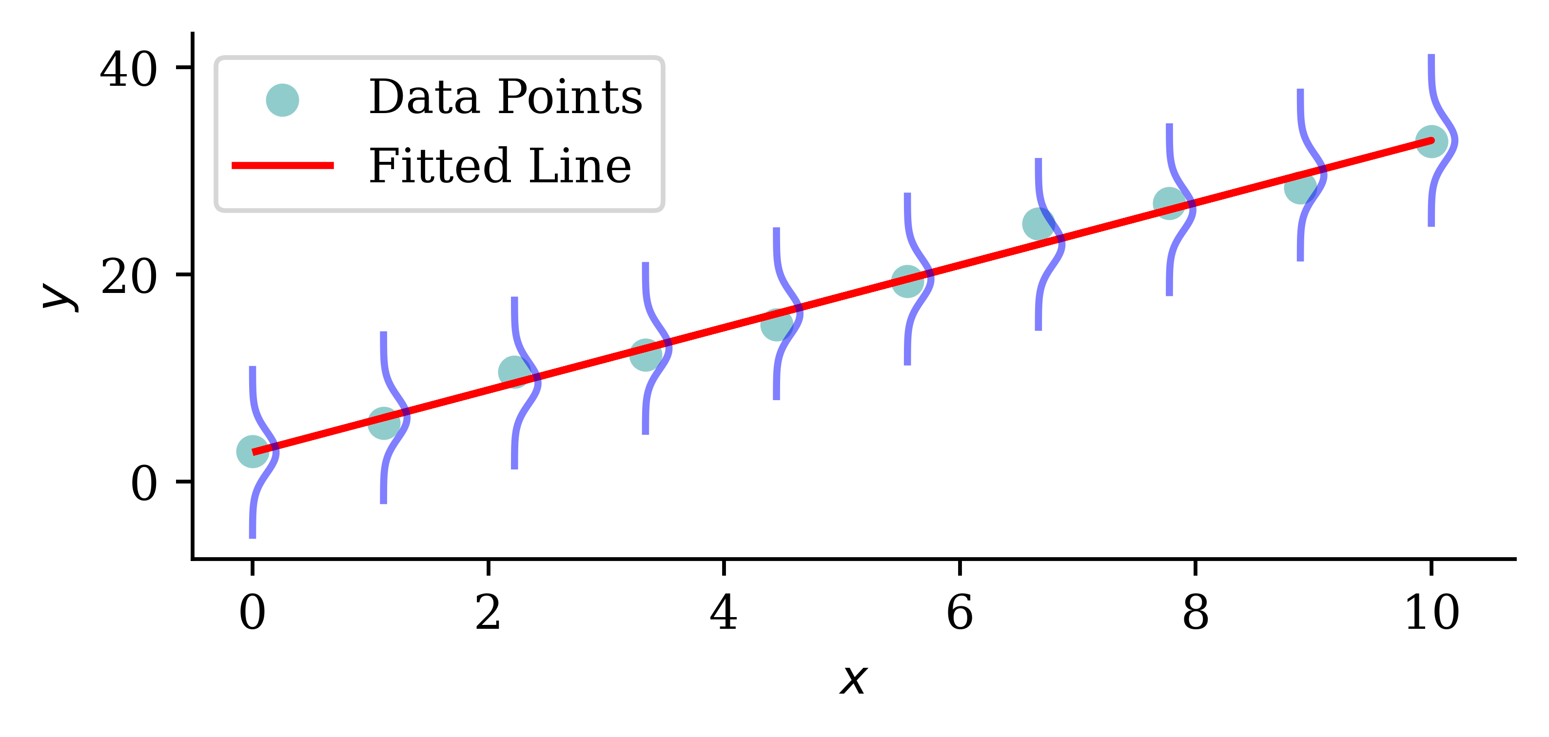
Visualising the distribution of each Y

Code
# Generate sample data for linear regression
np.random.seed(0)
X_toy = np.linspace(0, 10, 10)
np.random.shuffle(X_toy)

beta_0 = 2
beta_1 = 3
y_toy = beta_0 + beta_1 * X_toy + np.random.normal(scale=2, size=X_toy.shape)
sigma_toy = 2  # Assuming a standard deviation for the normal distribution

# Fit a simple linear regression model
coefficients = np.polyfit(X_toy, y_toy, 1)
predicted_y = np.polyval(coefficients, X_toy)

# Plot the data points and the fitted line
plt.scatter(X_toy, y_toy, label='Data Points')
plt.plot(X_toy, predicted_y, color='red', label='Fitted Line')

# Draw the normal distribution bell curve sideways at each data point
for i in range(len(X_toy)):
    mu = predicted_y[i]
    y_values = np.linspace(mu - 4*sigma_toy, mu + 4*sigma_toy, 100)
    x_values = stats.norm.pdf(y_values, mu, sigma_toy) + X_toy[i]
    plt.plot(x_values, y_values, color='blue', alpha=0.5)

plt.xlabel('$x$')
plt.ylabel('$y$')
plt.legend()
The probabilistic view

Y_i \sim \mathcal{N}(\mu_i, \sigma^2)

where \mu_i = \beta_0 + \beta_1 x_{i1} + \ldots + \beta_p x_{ip}, and the \sigma^2 is known.

The \mathcal{N}(\mu, \sigma^2) normal distribution has p.d.f.

f(y) = \frac{1}{\sqrt{2\pi\sigma^2}} \exp\left(-\frac{(y - \mu)^2}{2\sigma^2}\right) .

The likelihood function is

L(\boldsymbol{\beta}) = \prod_{i=1}^n \frac{1}{\sqrt{2\pi\sigma^2}} \exp\left(-\frac{(y_i - \mu_i)^2}{2\sigma^2}\right) \Rightarrow \ell(\boldsymbol{\beta}) = -\frac{n}{2}\log(2\pi) - \frac{n}{2}\log(\sigma^2) - \frac{1}{2\sigma^2}\sum_{i=1}^n (y_i - \mu_i)^2 .

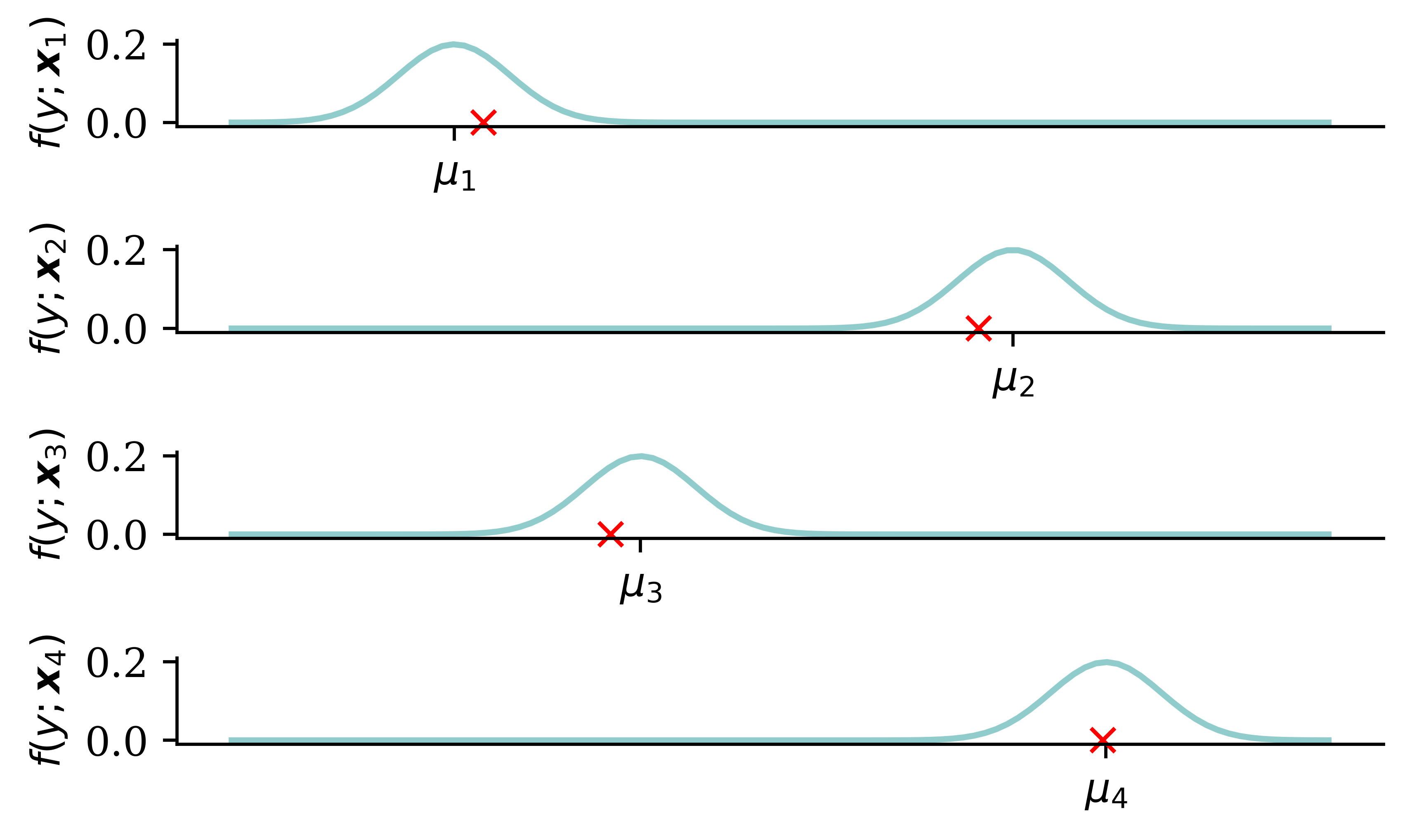
Perform maximum likelihood estimation to find \boldsymbol{\beta}.

The predicted distributions

Code
y_pred = np.polyval(coefficients, X_toy[:4])

fig, axes = plt.subplots(4, 1, figsize=(5.0, 3.0))

x_min = y_pred[:4].min() - 4*sigma_toy
x_max = y_pred[:4].max() + 4*sigma_toy
x_grid = np.linspace(x_min, x_max, 100)

# Plot each normal distribution with different means vertically
for i, ax in enumerate(axes):
    mu = y_pred[i]
    y_grid = stats.norm.pdf(x_grid, mu, sigma_toy)
    ax.plot(x_grid, y_grid)
    ax.set_ylabel(f'$f(y ; \\boldsymbol{{x}}_{{{i+1}}})$')
    ax.set_xticks([y_pred[i]], labels=[r'$\mu_{' + str(i+1) + r'}$'])
    ax.plot(y_toy[i], 0, 'rx', clip_on=False)

plt.tight_layout();
The machine learning view

The negative log-likelihood \text{NLL}(\boldsymbol{\beta}) := -\ell(\boldsymbol{\beta}) is to be minimised:

\text{NLL}(\boldsymbol{\beta}) = \frac{n}{2}\log(2\pi) + \frac{n}{2}\log(\sigma^2) + \frac{1}{2\sigma^2}\sum_{i=1}^n (y_i - \mu_i)^2 .

As \sigma^2 is fixed, minimising NLL is equivalent to minimising MSE:

\begin{aligned} \boldsymbol{\beta}^* &= \underset{\boldsymbol{\beta}}{\operatorname{arg\,min}}\,\, \text{NLL}(\boldsymbol{\beta}) \\ &= \underset{\boldsymbol{\beta}}{\operatorname{arg\,min}}\,\, \frac{n}{2}\log(2\pi) + \frac{n}{2}\log(\sigma^2) + \frac{1}{2\sigma^2}\sum_{i=1}^n (y_i - \mu_i)^2 \\ &= \underset{\boldsymbol{\beta}}{\operatorname{arg\,min}}\,\, \frac{1}{n} \sum_{i=1}^n \Bigl( y_i - \hat{y}_i(\boldsymbol{x}_i; \boldsymbol{\beta}) \Bigr)^2 \\ &= \underset{\boldsymbol{\beta}}{\operatorname{arg\,min}}\,\, \text{MSE}\bigl( \boldsymbol{y}, \hat{\boldsymbol{y}}(\mathbf{X}; \boldsymbol{\beta}) \bigr). \end{aligned}

Generalised Linear Model (GLM)

The GLM is often characterised by the mean prediction:

\mu(\boldsymbol{x}; \boldsymbol{\beta}) = g^{-1} \left(\left\langle \boldsymbol{\beta}, \boldsymbol{x} \right\rangle\right)

where g is the link function.

Common GLM distributions for the response variable include:

  • Normal distribution with identity link (just MLR)
  • Bernoulli distribution with logit link (logistic regression)
  • Poisson distribution with log link (Poisson regression)
  • Gamma distribution with log link

Logistic regression

A Bernoulli distribution with parameter p has p.m.f.

f(y)\ =\ \begin{cases} p & \text{if } y = 1 \\ 1 - p & \text{if } y = 0 \end{cases} \ =\ p^y (1 - p)^{1 - y}.

Our model is Y|\boldsymbol{X}=\boldsymbol{x} follows a Bernoulli distribution with parameter

\mu(\boldsymbol{x}; \boldsymbol{\beta}) = \frac{1}{1 + \exp\left(-\left\langle \boldsymbol{\beta}, \boldsymbol{x} \right\rangle\right)} = \mathbb{P}(Y=1|\boldsymbol{X}=\boldsymbol{x}).

The likelihood function, using \mu_i := \mu(\boldsymbol{x}_i; \boldsymbol{\beta}), is

L(\boldsymbol{\beta}) \ =\ \prod_{i=1}^n \begin{cases} \mu_i & \text{if } y_i = 1 \\ 1 - \mu_i & \text{if } y_i = 0 \end{cases} \ =\ \prod_{i=1}^n \mu_i^{y_i} (1 - \mu_i)^{1 - y_i} .

Binary cross-entropy loss

L(\boldsymbol{\beta}) = \prod_{i=1}^n \mu_i^{y_i} (1 - \mu_i)^{1 - y_i} \Rightarrow \ell(\boldsymbol{\beta}) = \sum_{i=1}^n \Bigl( y_i \log(\mu_i) + (1 - y_i) \log(1 - \mu_i) \Bigr).

The negative log-likelihood is

\text{NLL}(\boldsymbol{\beta}) = -\sum_{i=1}^n \Bigl( y_i \log(\mu_i) + (1 - y_i) \log(1 - \mu_i) \Bigr).

The binary cross-entropy loss is basically identical: \text{BCE}(\boldsymbol{y}, \boldsymbol{\mu}) = - \frac{1}{n} \sum_{i=1}^n \Bigl( y_i \log(\mu_i) + (1 - y_i) \log(1 - \mu_i) \Bigr).

Poisson regression

A Poisson distribution with rate \lambda has p.m.f. f(y) = \frac{\lambda^y \exp(-\lambda)}{y!}.

Our model is Y|\boldsymbol{X}=\boldsymbol{x} is Poisson distributed with parameter

\mu(\boldsymbol{x}; \boldsymbol{\beta}) = \exp\left(\left\langle \boldsymbol{\beta}, \boldsymbol{x} \right\rangle\right) .

The likelihood function is

L(\boldsymbol{\beta}) = \prod_{i=1}^n \frac{ \mu_i^{y_i} \exp(-\mu_i) }{y_i!} \Rightarrow \ell(\boldsymbol{\beta}) = \sum_{i=1}^n \Bigl( -\mu_i + y_i \log(\mu_i) - \log(y_i!) \Bigr).

Poisson loss

The negative log-likelihood is

\text{NLL}(\boldsymbol{\beta}) = \sum_{i=1}^n \Bigl( \mu_i - y_i \log(\mu_i) + \log(y_i!) \Bigr) .

The Poisson loss is

\text{Poisson}(\boldsymbol{y}, \boldsymbol{\mu}) = \frac{1}{n} \sum_{i=1}^n \Bigl( \mu_i - y_i \log(\mu_i) \Bigr).

Gamma regression

A Gamma distribution with mean \mu and dispersion \phi has p.d.f. f(y; \mu, \phi) = \frac{(\mu \phi)^{-\frac{1}{\phi}}}{\Gamma\left(\frac{1}{\phi}\right)} y^{\frac{1}{\phi} - 1} \mathrm{e}^{-\frac{y}{\mu \phi}}

Our model is Y|\boldsymbol{X}=\boldsymbol{x} is Gamma distributed with a dispersion of \phi and a mean of \mu(\boldsymbol{x}; \boldsymbol{\beta}) = \exp\left(\left\langle \boldsymbol{\beta}, \boldsymbol{x} \right\rangle\right).

The likelihood function is L(\boldsymbol{\beta}) = \prod_{i=1}^n \frac{(\mu_i \phi)^{-\frac{1}{\phi}}}{\Gamma\left(\frac{1}{\phi}\right)} y_i^{\frac{1}{\phi} - 1} \exp\left(-\frac{y_i}{\mu_i \phi}\right)

\Rightarrow \ell(\boldsymbol{\beta}) = \sum_{i=1}^n \left[ -\frac{1}{\phi} \log(\mu_i \phi) - \log \Gamma\left(\frac{1}{\phi}\right) + \left(\frac{1}{\phi} - 1\right) \log(y_i) - \frac{y_i}{\mu_i \phi} \right].

Gamma loss

The negative log-likelihood is

\text{NLL}(\boldsymbol{\beta}) = \sum_{i=1}^n \left[ \frac{1}{\phi} \log(\mu_i \phi) + \log \Gamma\left(\frac{1}{\phi}\right) - \left(\frac{1}{\phi} - 1\right) \log(y_i) + \frac{y_i}{\mu_i \phi} \right].

Since \phi is a nuisance parameter \text{NLL}(\boldsymbol{\beta}) = \sum_{i=1}^n \left[ \frac{1}{\phi} \log(\mu_i) + \frac{y_i}{\mu_i \phi} \right] + \text{const} \propto \sum_{i=1}^n \left[ \log(\mu_i) + \frac{y_i}{\mu_i} \right].

Note

As \log(\mu_i) = \log(y_i) - \log(y_i / \mu_i), we could write an alternative version \text{NLL}(\boldsymbol{\beta}) \propto \sum_{i=1}^n \left[ \log(y_i) - \log\Bigl(\frac{y_i}{\mu_i}\Bigr) + \frac{y_i}{\mu_i} \right] \propto \sum_{i=1}^n \left[ \frac{y_i}{\mu_i} - \log\Bigl(\frac{y_i}{\mu_i}\Bigr) \right].

Why do actuaries use GLMs?

  • GLMs are interpretable.
  • GLMs are flexible (can handle different types of response variables).
  • We get the full distribution of the response variable, not just the mean.

This last point is particularly important for analysing worst-case scenarios.

Stochastic Forecasts

Lecture Outline

  • Introduction

  • Traditional Regression

  • Stochastic Forecasts

  • GLMs and Neural Networks

  • Combined Actuarial Neural Network

  • Mean-Variance Estimation Network

  • Mixture Density Network

  • Distributional Refinement Network

  • Uncertainty and Regularisation

  • Dropout and Ensembles

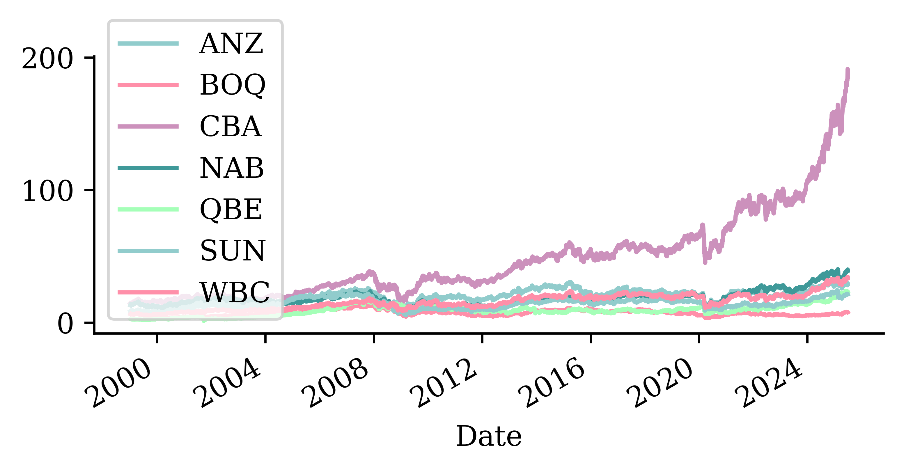
Stock price forecasting

Code
def lagged_timeseries(df, target, window):
    lagged = pd.DataFrame()
    for i in range(window, 0, -1):
        lagged[f"T-{i}"] = df[target].shift(i)
    lagged["T"] = df[target].values
    return lagged


stocks = pd.read_csv("data/interim/aus_fin_stocks.csv")
stocks["Date"] = pd.to_datetime(stocks["Date"])
stocks = stocks.set_index("Date")
_ = stocks.pop("ASX200")
stock = stocks[["CBA"]]
stock = stock.ffill()

# Compute daily log returns
stock_log = np.log(stock / stock.shift(1)).dropna()

# Helper functions for converting log returns to prices
def log_to_price(log_returns, initial_price):
    cumulative_log_returns = log_returns.cumsum()
    return initial_price * np.exp(cumulative_log_returns)

def get_last_price(stock_df, cutoff_date):
    last_known_date = stock_df.loc[:cutoff_date].index[-1]
    return stock_df.loc[last_known_date, "CBA"]

# Create lagged features from log returns
df_lags = lagged_timeseries(stock_log, "CBA", 40)

# Split the data in time (same cutoffs as the Time Series lecture)
X_train = df_lags.loc[:"2014"]
X_val = df_lags.loc["2015":"2020"]
X_test = df_lags.loc["2021":]

# Remove any with NAs and split into X and y
X_train = X_train.dropna()
X_val = X_val.dropna()
X_test = X_test.dropna()

y_train = X_train.pop("T")
y_val = X_val.pop("T")
y_test = X_test.pop("T")

lr = LinearRegression()
lr.fit(X_train, y_train);
Code
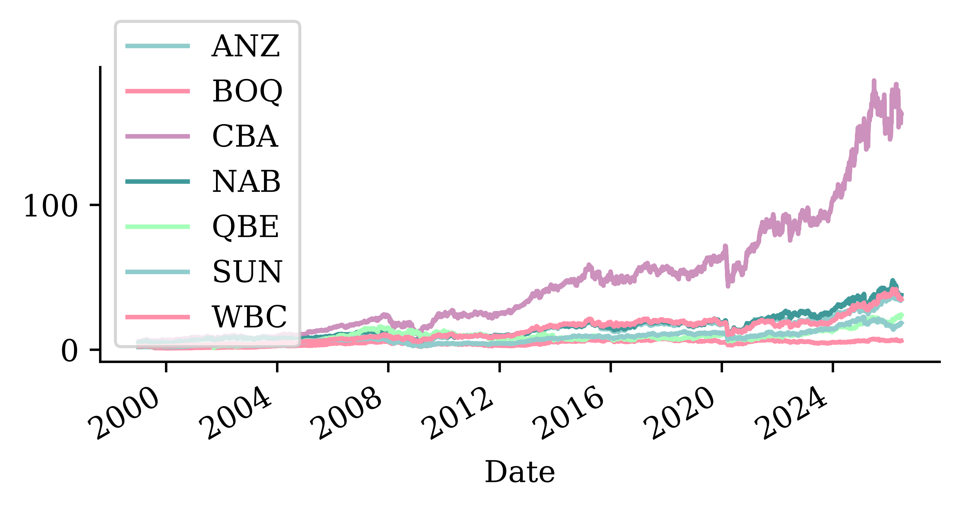
stocks.plot();

Code
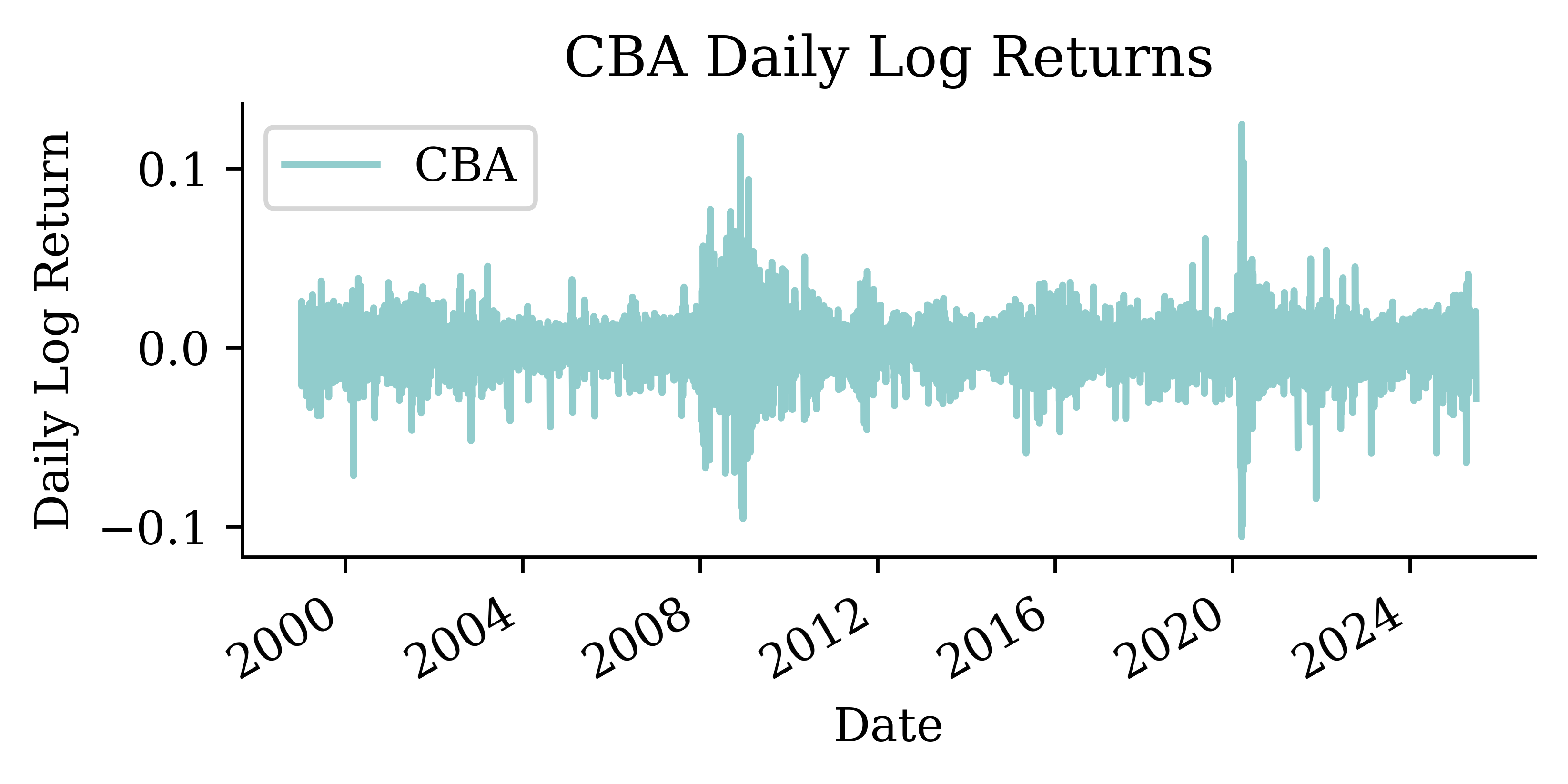
stock_log.plot()
plt.ylabel("Daily Log Return")
plt.title("CBA Daily Log Returns");

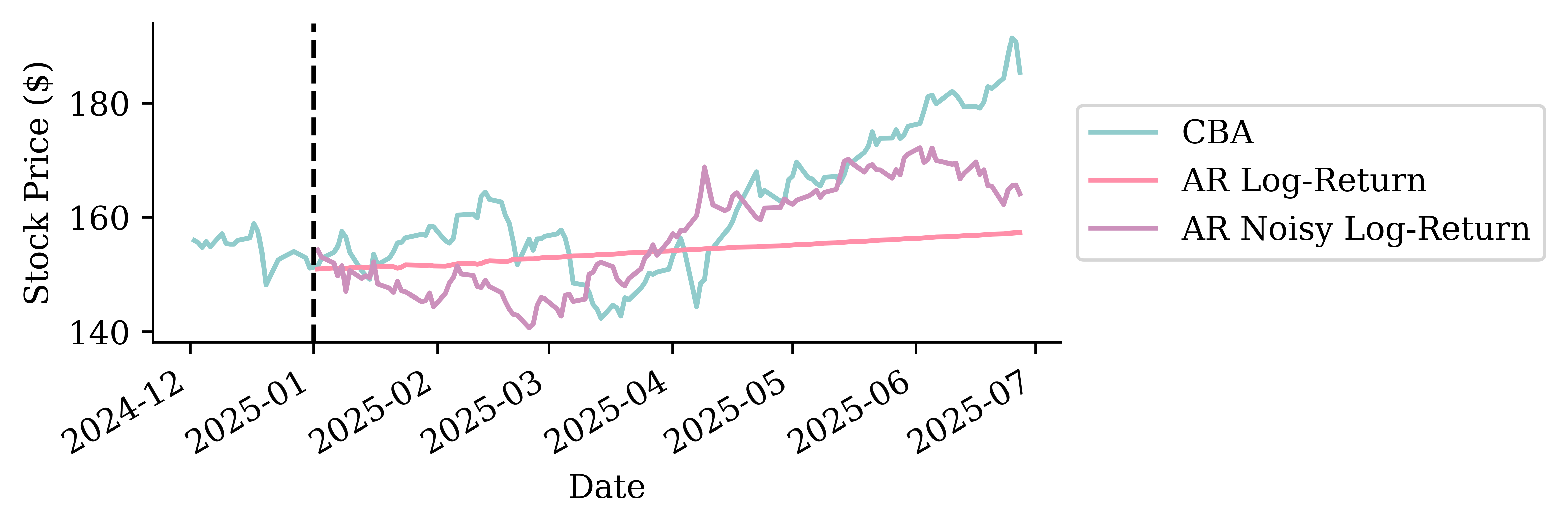
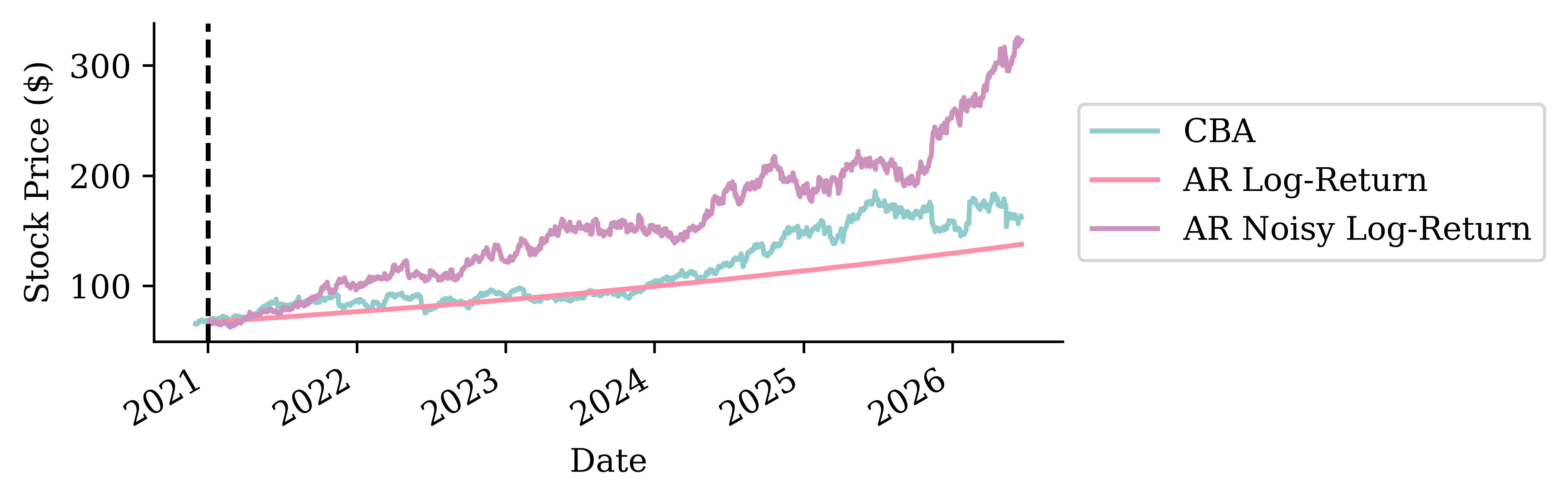
Noisy auto-regressive forecast

def noisy_autoregressive_forecast(model, X_val, sigma):
    """Roll a one-step model forward, feeding each (noisy) prediction back in."""
    window = np.asarray(X_val.iloc[0], dtype="float32").copy()
    preds = []
    for _ in range(len(X_val)):
        X_next = pd.DataFrame(window.reshape(1, -1), columns=X_val.columns)
        next_value = model.predict(X_next).flatten()[0]
        next_value += np.random.normal(0, sigma)
        preds.append(next_value)
        window = np.append(window[1:], next_value)  # drop oldest, add prediction
    return pd.Series(preds, index=X_val.index, name="Multi Step")

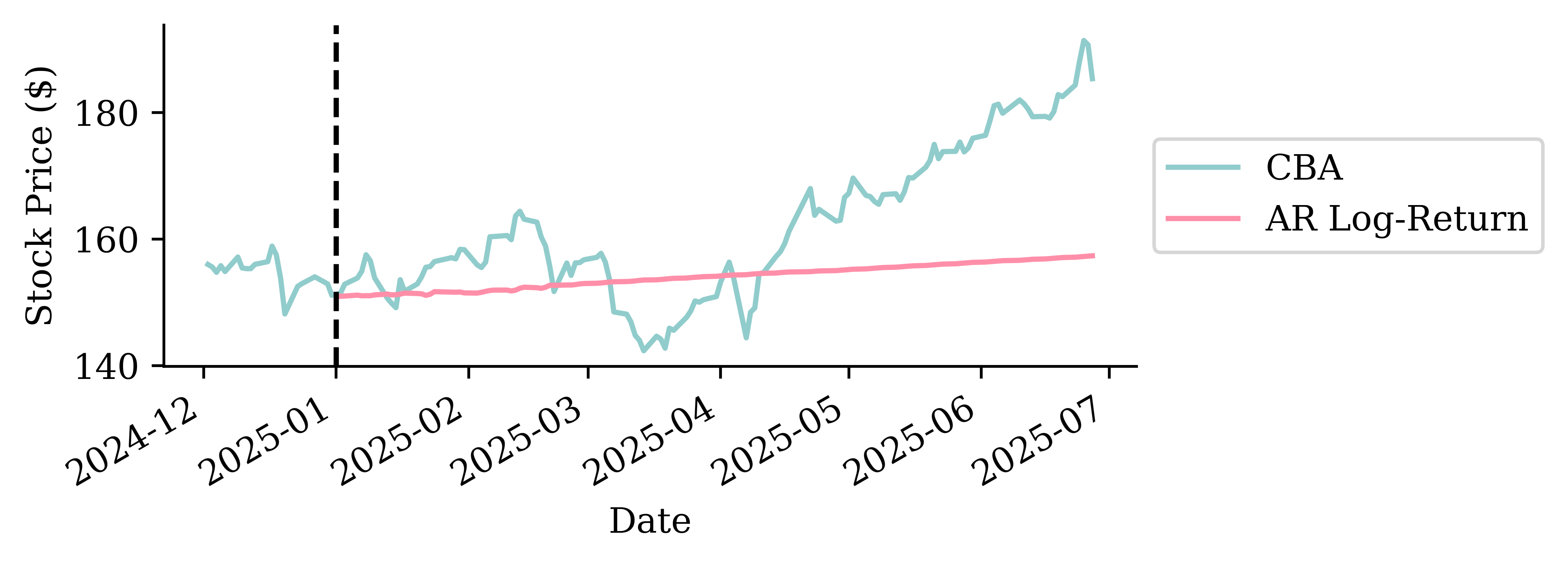
Original forecast

lr_forecast = noisy_autoregressive_forecast(lr, X_test, 0)
last_price = get_last_price(stock, cutoff_date="2020-12")
price_forecast = log_to_price(lr_forecast, last_price)
Code
stock.loc[price_forecast.index, "AR Log-Return"] = price_forecast

def plot_forecasts(stock):
    stock.loc["2020-12":].plot()
    plt.axvline("2021", color="black", linestyle="--")
    plt.ylabel("Stock Price ($)")
    plt.legend(loc="center left", bbox_to_anchor=(1, 0.5))

plot_forecasts(stock)

residuals = y_val - lr.predict(X_val)
sigma = np.std(residuals)

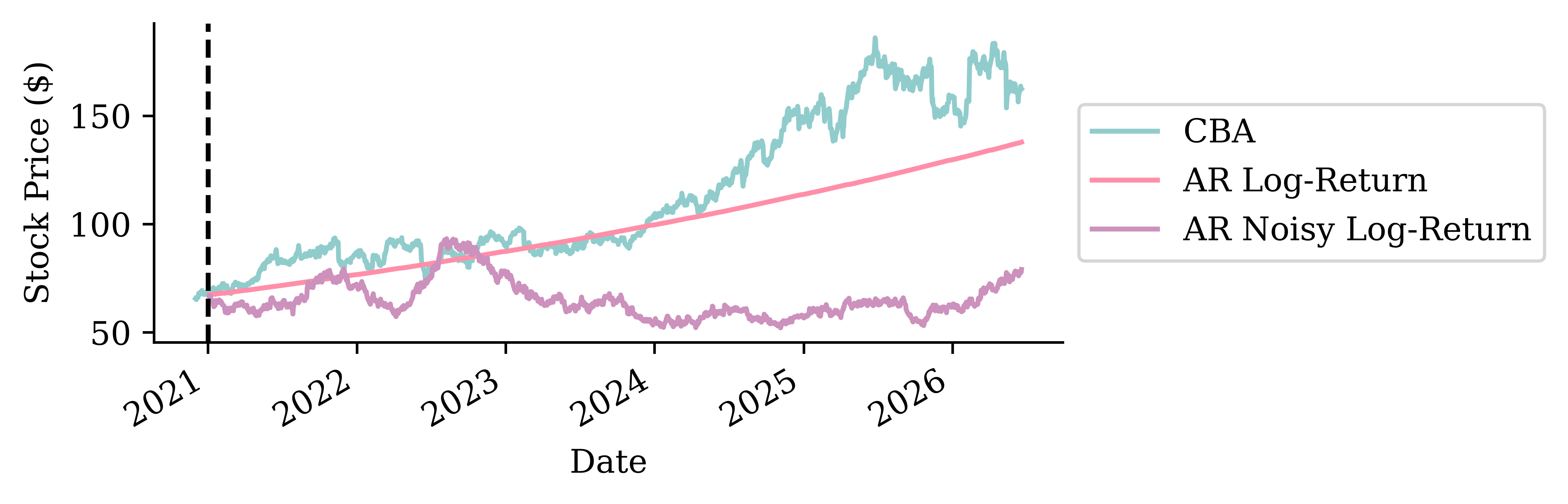
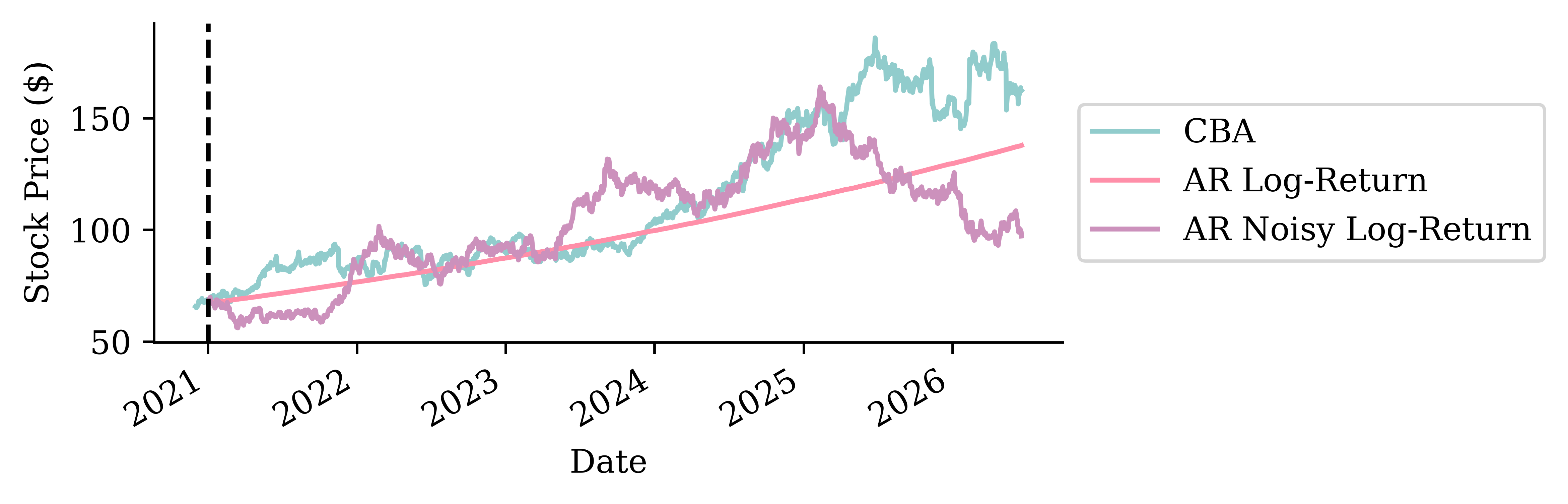
With noise

np.random.seed(1)
lr_noisy_forecast = noisy_autoregressive_forecast(lr, X_test, sigma)
price_noisy = log_to_price(lr_noisy_forecast, last_price)
Code
stock.loc[price_noisy.index, "AR Noisy Log-Return"] = price_noisy
plot_forecasts(stock)

With noise

np.random.seed(2)
lr_noisy_forecast = noisy_autoregressive_forecast(lr, X_test, sigma)
price_noisy = log_to_price(lr_noisy_forecast, last_price)
Code
stock.loc[price_noisy.index, "AR Noisy Log-Return"] = price_noisy
plot_forecasts(stock)

With noise

np.random.seed(3)
lr_noisy_forecast = noisy_autoregressive_forecast(lr, X_test, sigma)
price_noisy = log_to_price(lr_noisy_forecast, last_price)
Code
stock.loc[price_noisy.index, "AR Noisy Log-Return"] = price_noisy
plot_forecasts(stock)

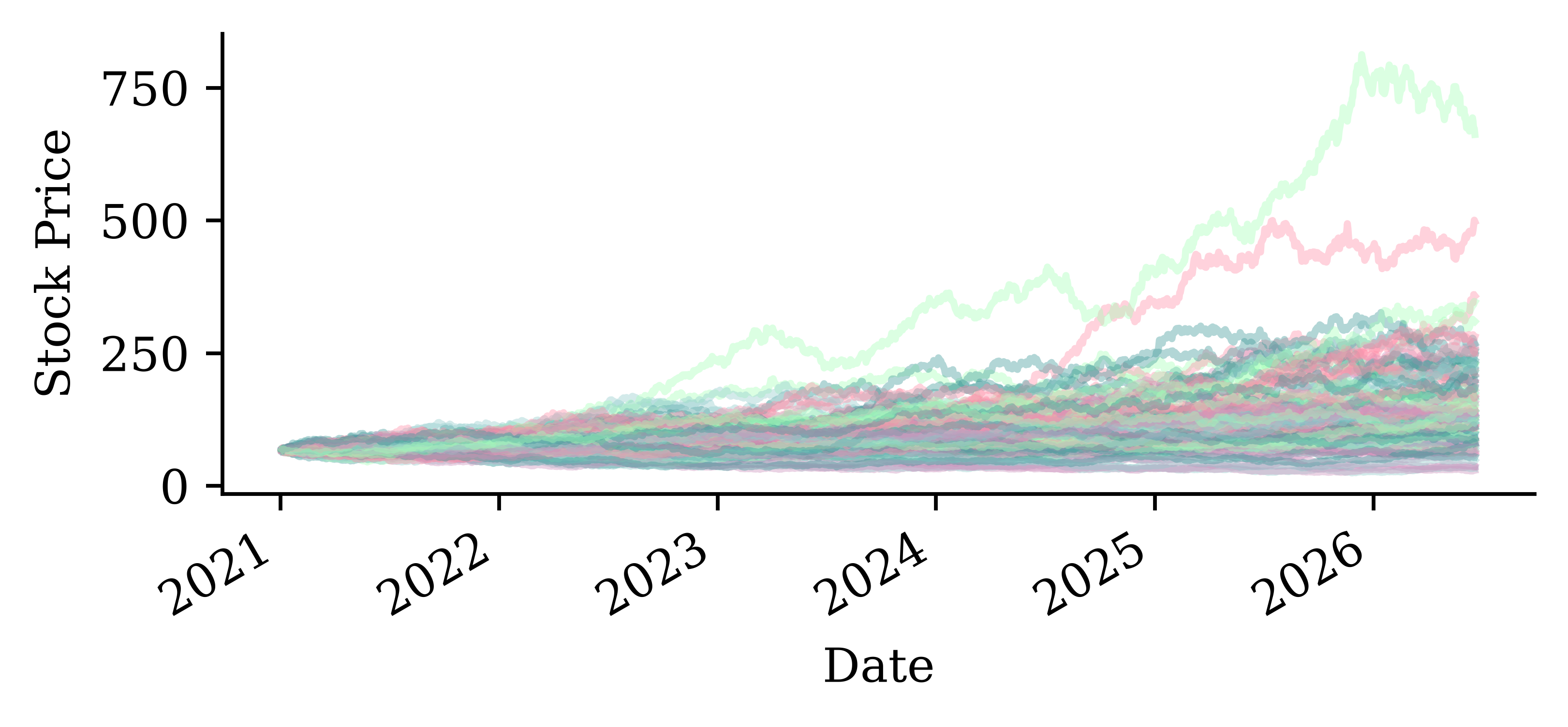
Many noisy forecasts

num_forecasts = 100
forecasts = []
for i in range(num_forecasts):
    sim = log_to_price(noisy_autoregressive_forecast(lr, X_test, sigma), last_price)
    forecasts.append(sim)
noisy_forecasts = pd.concat(forecasts, axis=1)
noisy_forecasts.index = X_test.index
Code
noisy_forecasts.plot(legend=False, alpha=0.4)
plt.ylabel("Stock Price");

95% β€œprediction intervals”

# Calculate quantiles for the forecasts
lower_quantile = noisy_forecasts.quantile(0.025, axis=1)
upper_quantile = noisy_forecasts.quantile(0.975, axis=1)
mean_forecast = noisy_forecasts.mean(axis=1)
Code
# Plot the mean forecast
plt.figure(figsize=(8, 3))

plt.plot(stock.loc["2020-12":].index, stock.loc["2020-12":]["CBA"], label="CBA")

plt.plot(mean_forecast, label="Mean")

# Plot the quantile-based shaded area
plt.fill_between(mean_forecast.index, 
                 lower_quantile, 
                 upper_quantile, 
                 color="grey", alpha=0.2)

# Plot settings
plt.axvline(pd.Timestamp("2021-01-01"), color="black", linestyle="--")
plt.legend(loc="center left", bbox_to_anchor=(1, 0.5))
plt.xlabel("Date")
plt.ylabel("Stock Price")
plt.tight_layout();
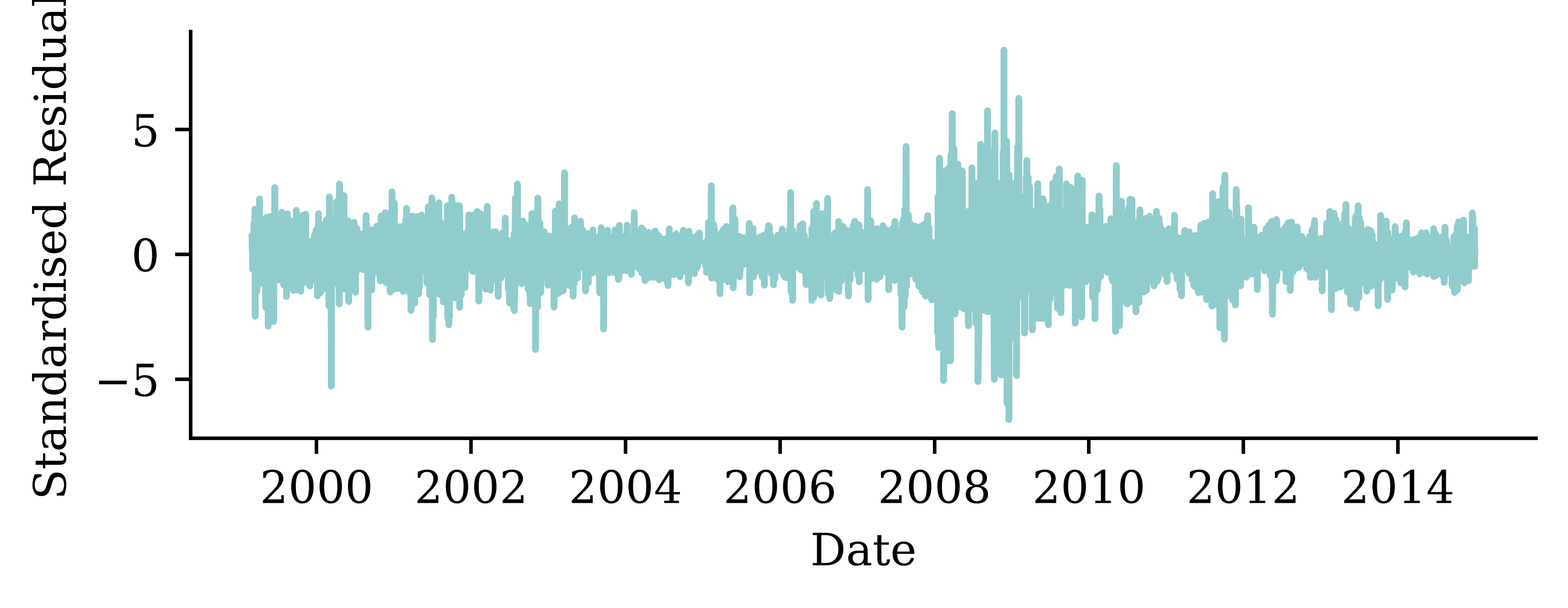
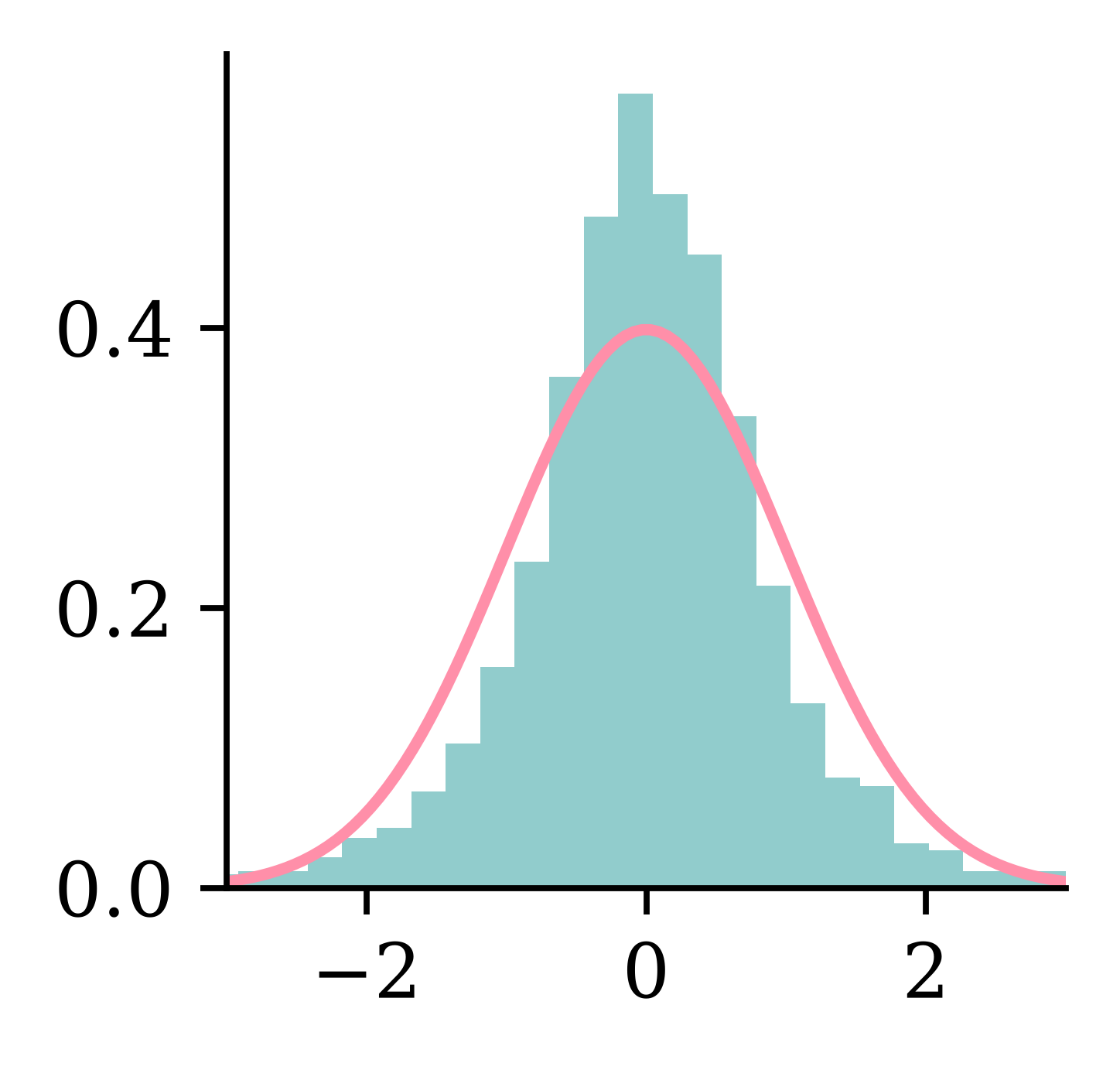
Residuals
y_pred = lr.predict(X_train)
residuals = y_train - y_pred
residuals -= np.mean(residuals)
residuals /= np.std(residuals)
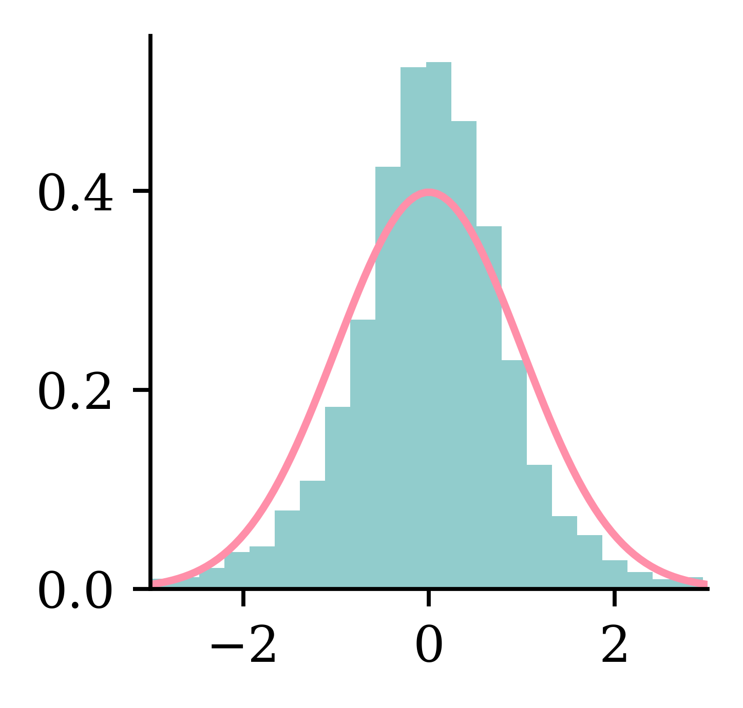
stats.shapiro(residuals)
ShapiroResult(statistic=np.float64(0.939218900099982), pvalue=np.float64(6.991031400920509e-38))
Code
plt.hist(residuals, bins=60, density=True)
x = np.linspace(-3, 3, 100)
plt.xlim(-3, 3)
plt.plot(x, stats.norm.pdf(x, 0, 1));

Q-Q plot and P-P plot

Code
sm.qqplot(residuals, line="45");

Code
sm.ProbPlot(residuals).ppplot(line="45");

Residuals against time

Code
plt.plot(y_train.index, residuals)
plt.xlabel("Date")
plt.ylabel("Standardised Residuals")
plt.tight_layout();

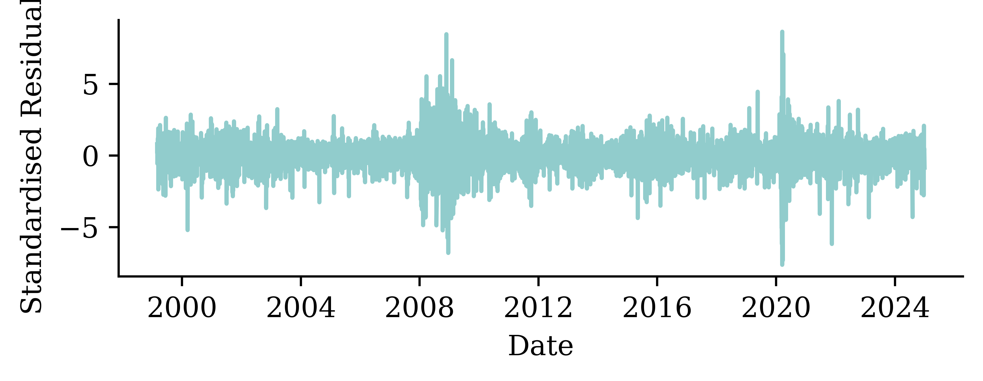
Heteroskedasticity!

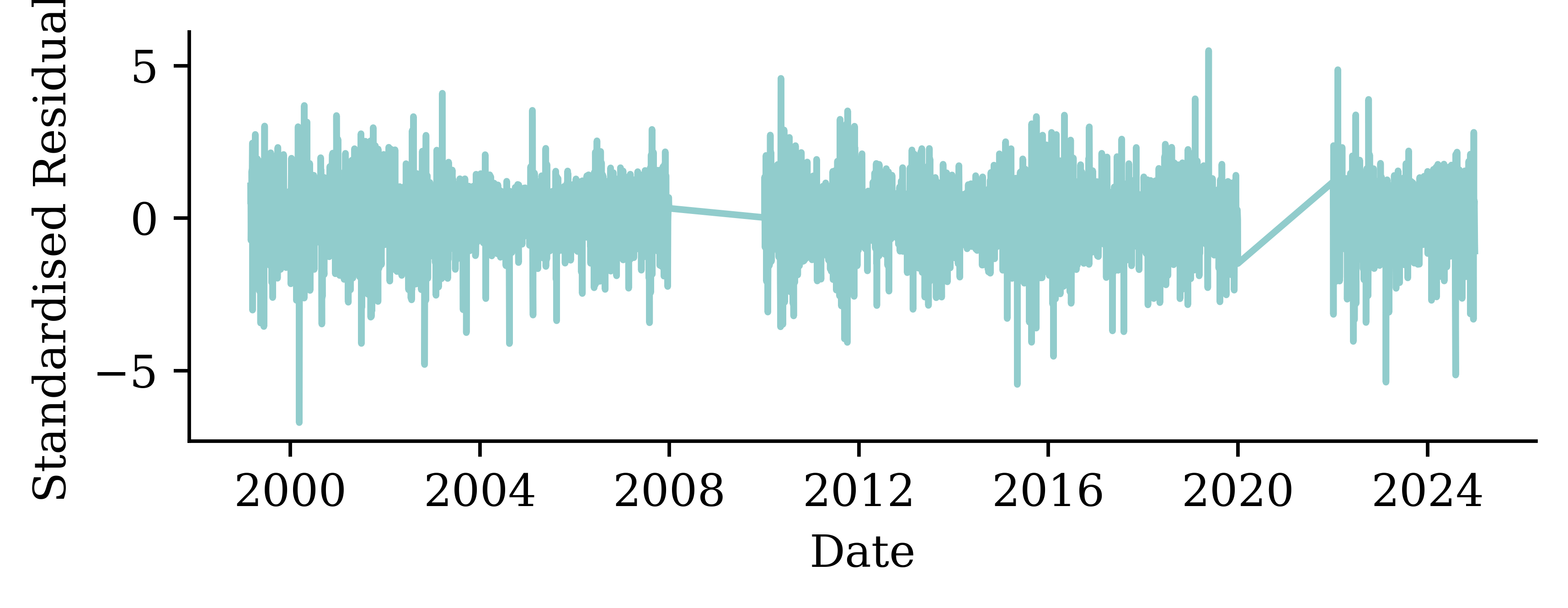
Retrain on less data

Code
# Drop the GFC years (2008-2009) from the training set
mask = ~((y_train.index.year >= 2008) & (y_train.index.year <= 2009))
X2 = X_train.loc[mask]
y2 = y_train.loc[mask]

lr2 = LinearRegression()
lr2.fit(X2, y2)

res2 = y2 - lr2.predict(X2)
res2 = (res2 - np.mean(res2)) / np.std(res2)

plt.plot(y2.index, res2)
plt.xlabel("Date")
plt.ylabel("Standardised Residuals")
plt.tight_layout();
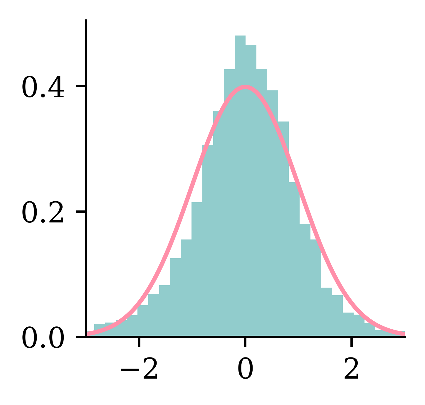
Refit the model without the GFC crisis years.

Residual diagnostics

stats.shapiro(res2)
ShapiroResult(statistic=np.float64(0.983029219714092), pvalue=np.float64(3.326265726133293e-20))
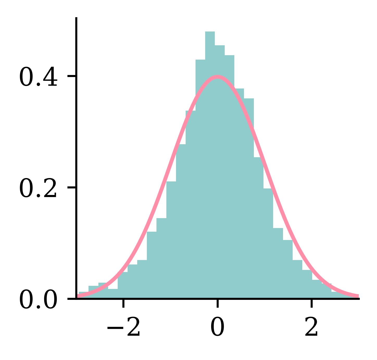
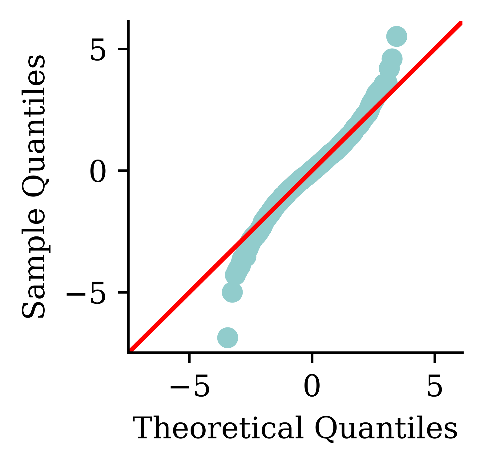
Code
plt.hist(res2, bins=60, density=True)
x = np.linspace(-3, 3, 100)
plt.xlim(-3, 3)
plt.plot(x, stats.norm.pdf(x, 0, 1));

Code
sm.qqplot(res2, line="45");

Code
sm.ProbPlot(res2).ppplot(line="45");

GLMs and Neural Networks

Lecture Outline

  • Introduction

  • Traditional Regression

  • Stochastic Forecasts

  • GLMs and Neural Networks

  • Combined Actuarial Neural Network

  • Mean-Variance Estimation Network

  • Mixture Density Network

  • Distributional Refinement Network

  • Uncertainty and Regularisation

  • Dropout and Ensembles

French motor claim sizes

sev = pd.read_csv('data/freMTPL2sev.csv')
cov = pd.read_csv('data/freMTPL2freq.csv').drop(columns=['ClaimNb'])
sev = pd.merge(sev, cov, on='IDpol', how='left').drop(columns=["IDpol"]).dropna()
sev
ClaimAmount Exposure VehPower VehAge DrivAge BonusMalus VehBrand VehGas Area Density Region
0 995.20 0.59 11.0 0.0 39.0 56.0 B12 Diesel D 778.0 Picardie
1 1128.12 0.95 4.0 1.0 49.0 50.0 B12 Regular E 2354.0 Ile-de-France
... ... ... ... ... ... ... ... ... ... ... ...
26637 767.55 0.43 6.0 0.0 67.0 50.0 B2 Diesel C 142.0 Languedoc-Roussillon
26638 1500.00 0.28 7.0 2.0 36.0 60.0 B12 Diesel D 1732.0 Rhone-Alpes

26444 rows Γ— 11 columns

Preprocessing

X_train, X_test, y_train, y_test = train_test_split(
  sev.drop("ClaimAmount", axis=1), sev["ClaimAmount"], random_state=2023)
ct = make_column_transformer(
    (make_pipeline(OrdinalEncoder(), StandardScaler()), ["Area", "VehGas"]),
    ("drop", ["VehBrand", "Region"]), remainder=StandardScaler())
X_train = ct.fit_transform(X_train)
X_test = ct.transform(X_test)
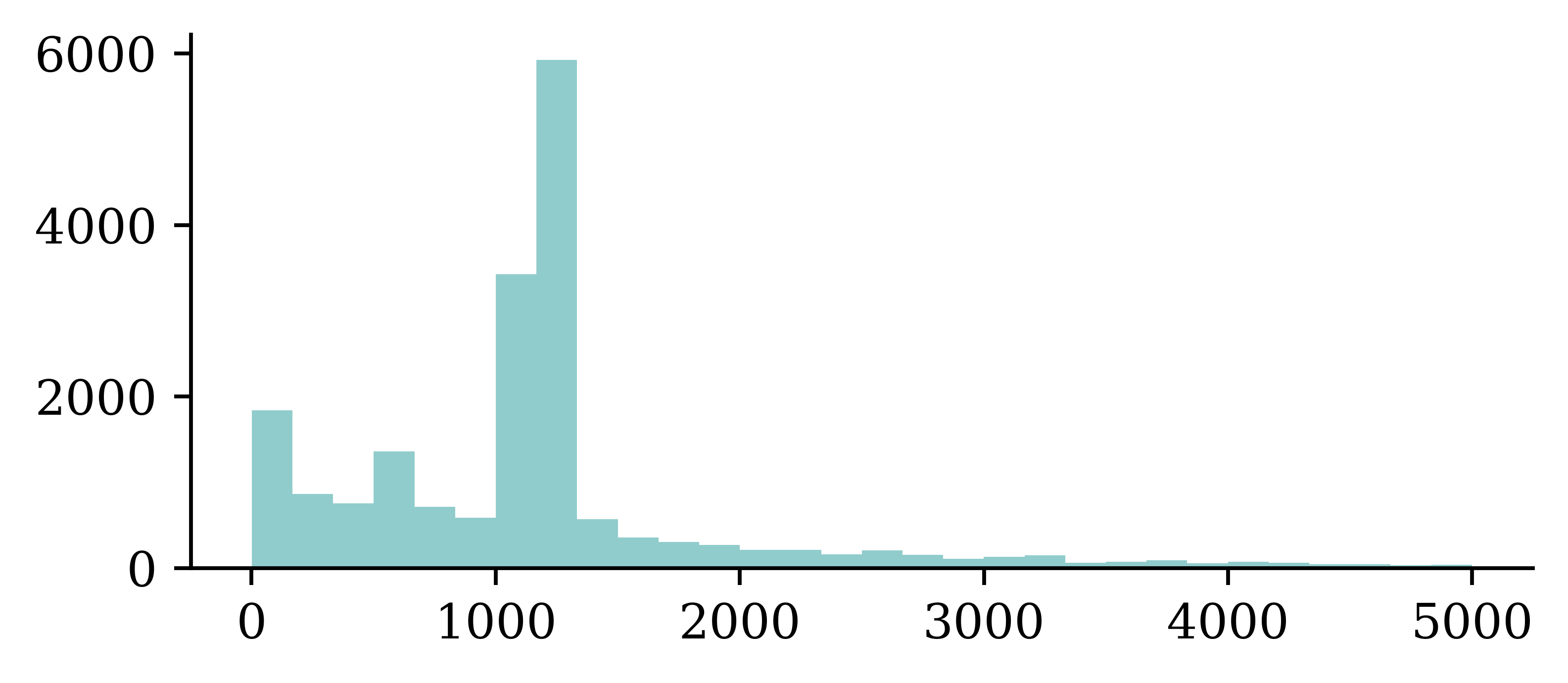
plt.hist(y_train[y_train < 5000], bins=30);
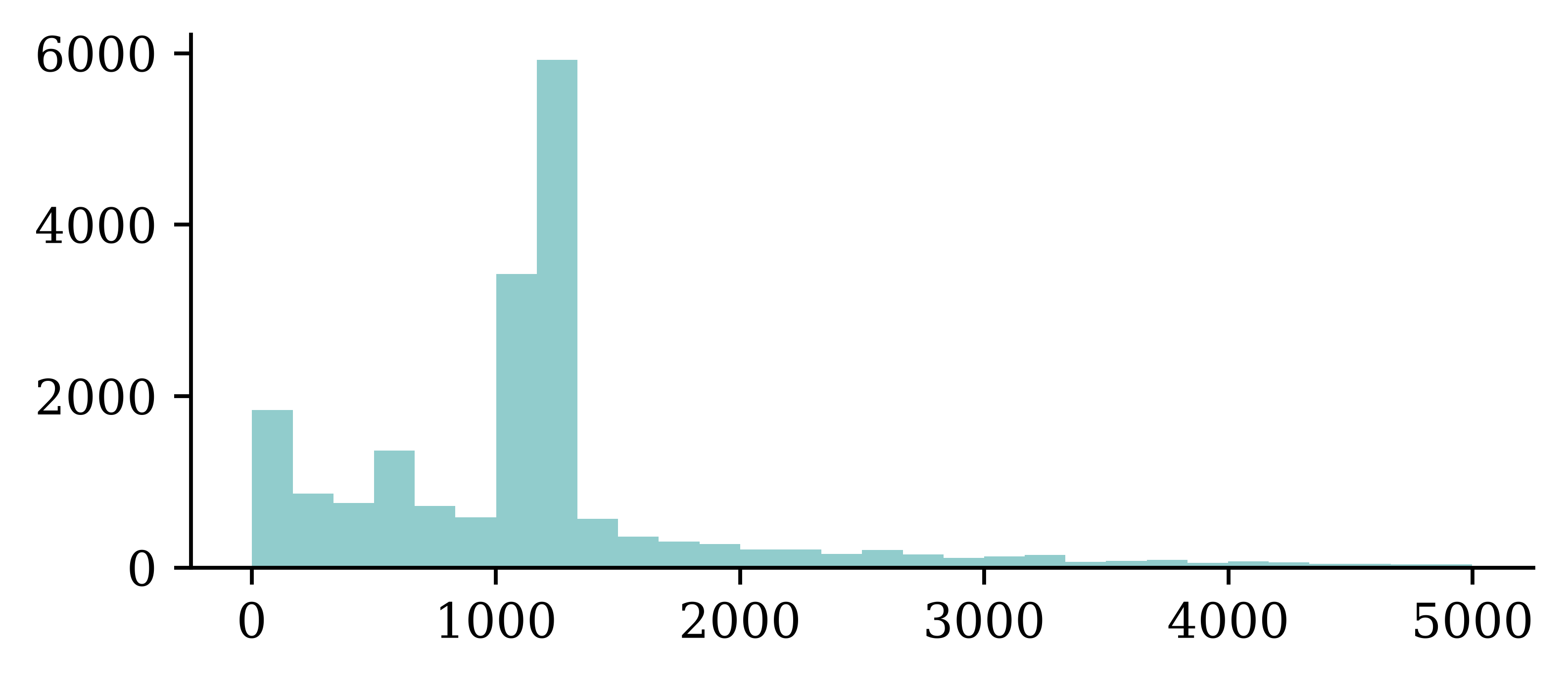
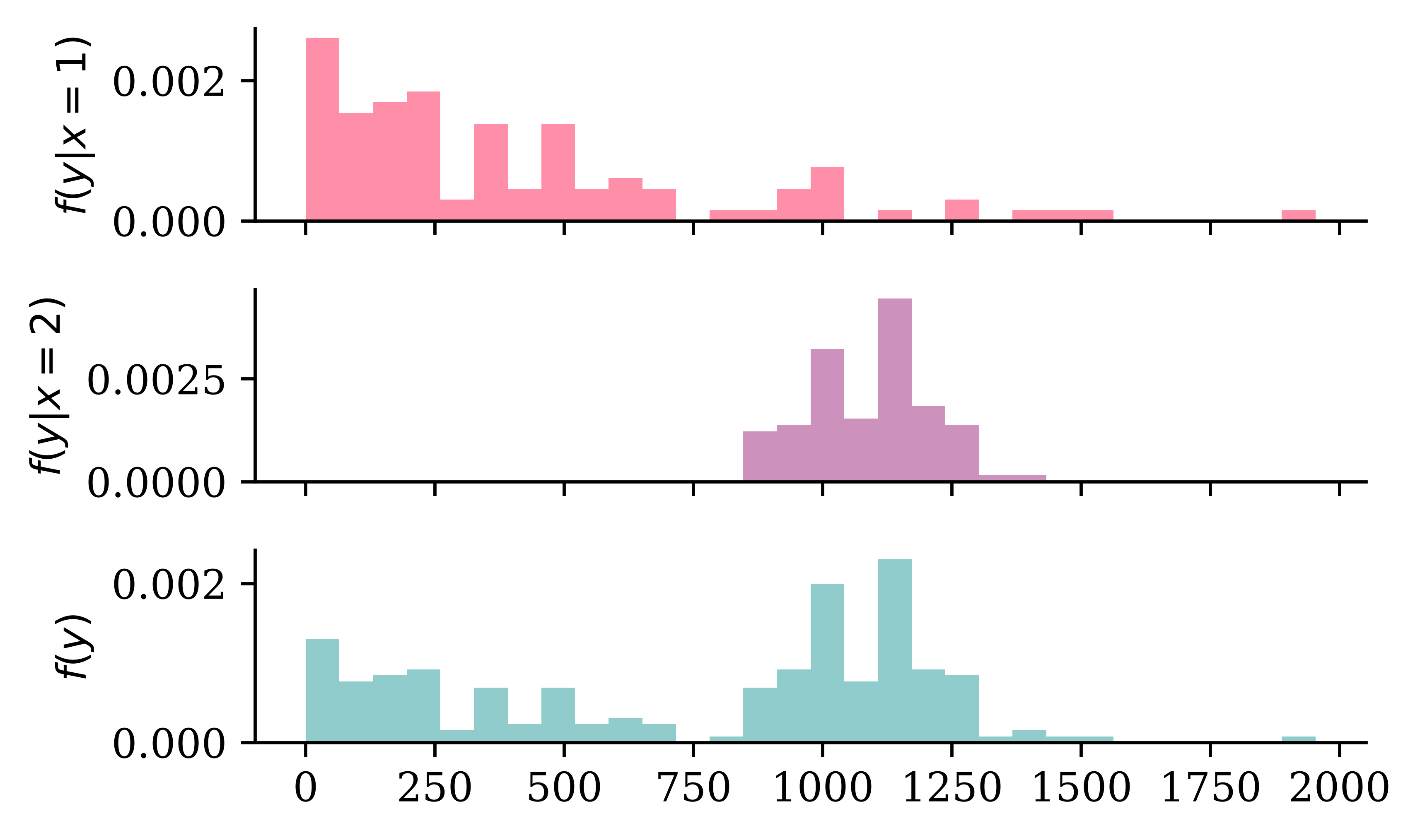
Doesn’t prove that Y | \boldsymbol{X} = \boldsymbol{x} is multimodal

Code
# Make some example where the distribution is multimodal because of a binary covariate which separates the means of the two distributions
np.random.seed(1)

fig, axes = plt.subplots(3, 1, figsize=(5.0, 3.0), sharex=True)

x_min = 0
x_max = y_train.max()
x_grid = np.linspace(x_min, x_max, 100)

# Simulate some data from an exponential distribution which has Pr(X < 1000) = 0.9
n = 100
p = 0.1
lambda_ = -np.log(p) / 1000 
mu = 1 / lambda_
y_1 = np.random.exponential(scale=mu, size=n)

# Pick a truncated normal distribution with a mean of 1100 and std of 250 (truncated to be positive)
mu = 1100
sigma = 100
y_2 = stats.truncnorm.rvs((0 - mu) / sigma, (np.inf - mu) / sigma, loc=mu, scale=sigma, size=n)

# Combine y_1 and y_2 for the final histogram
y = np.concatenate([y_1, y_2])

# Determine common bins
bins = np.histogram_bin_edges(y, bins=30)


# Plot each normal distribution with different means vertically
for i, ax in enumerate(axes):
    if i == 0:
        ax.hist(y_1, bins=bins, density=True, color=COLOURS[i+1])
        ax.set_ylabel(f'$f(y | x = 1)$')

    elif i == 1:
        ax.hist(y_2, bins=bins, density=True, color=COLOURS[i+1])
        ax.set_ylabel(f'$f(y | x = 2)$')

    else:
        ax.hist(y, bins=bins, density=True)
        ax.set_ylabel(f'$f(y)$')

plt.tight_layout();
Gamma GLM

Suppose a fitted Gamma GLM model has

  • a log link function g(x)=\log(x) and
  • regression coefficients \boldsymbol{\beta}=(\beta_0, \beta_1, \beta_2, \beta_3).

Then, it estimates the conditional mean of Y given a new instance \boldsymbol{x}=(1, x_1, x_2, x_3) as follows: \mathbb{E}[Y|\boldsymbol{X}=\boldsymbol{x}] = g^{-1}(\langle \boldsymbol{\beta}, \boldsymbol{x}\rangle) = \exp\big(\beta_0 + \beta_1 x_1 + \beta_2 x_2 + \beta_3 x_3 \big).

A GLM can model any other exponential family distribution using an appropriate link function g.

Gamma GLM loss

If Y|\boldsymbol{X}=\boldsymbol{x} is a Gamma r.v. with mean \mu(\boldsymbol{x}; \boldsymbol{\beta}) and dispersion parameter \phi, we can minimise the negative log-likelihood (NLL) \text{NLL} \propto \sum_{i=1}^{n}\left[ \log \mu (\boldsymbol{x}_i; \boldsymbol{\beta})+\frac{y_i}{\mu (\boldsymbol{x}_i; \boldsymbol{\beta})} \right] + \text{const}, i.e., we ignore the dispersion parameter \phi while estimating the regression coefficients.

What the GLM predicts

A GLM predicts the mean for each input; the dispersion is a single shared constant, estimated separately.
Fitting steps

Step 1. Use the advanced second derivative iterative method to find the regression coefficients: \boldsymbol{\beta}^* = \underset{\boldsymbol{\beta}}{\text{arg\,min}} \ \sum_{i=1}^{n}\left[ \log \mu (\boldsymbol{x}_i; \boldsymbol{\beta})+\frac{y_i}{\mu (\boldsymbol{x}_i; \boldsymbol{\beta})} \right]

Step 2. Estimate the dispersion parameter: \phi = \frac{1}{n-p}\sum_{i=1}^{n}\frac{\bigl(y_i-\mu(\boldsymbol{x}_i; \boldsymbol{\beta}^*)\bigr)^2}{\mu(\boldsymbol{x}_i; \boldsymbol{\beta}^* )^2}

(Here, p is the number of coefficients in the model. If this p doesn’t include the intercept, then the scaling should be \frac{1}{n-(p+1)}.)

Gamma GLM

In Python, we can fit a Gamma GLM as follows:

# Add a column of ones to include an intercept in the model
X_train_design = sm.add_constant(X_train)

# Create a Gamma GLM with a log link function
gamma_glm = sm.GLM(y_train, X_train_design,                   
            family=sm.families.Gamma(sm.families.links.Log()))

# Fit the model
gamma_glm = gamma_glm.fit()
gamma_glm.params
const                    7.648131
pipeline__Area          -0.099472
                           ...   
remainder__BonusMalus    0.157204
remainder__Density       0.010539
Length: 9, dtype: float64
# Dispersion Parameter
mus = gamma_glm.predict(X_train_design)
residuals = y_train - mus
dof = (len(y_train)-X_train_design.shape[1])
phi_glm = np.sum(residuals**2/mus**2)/dof
print(phi_glm)
59.63363123736379

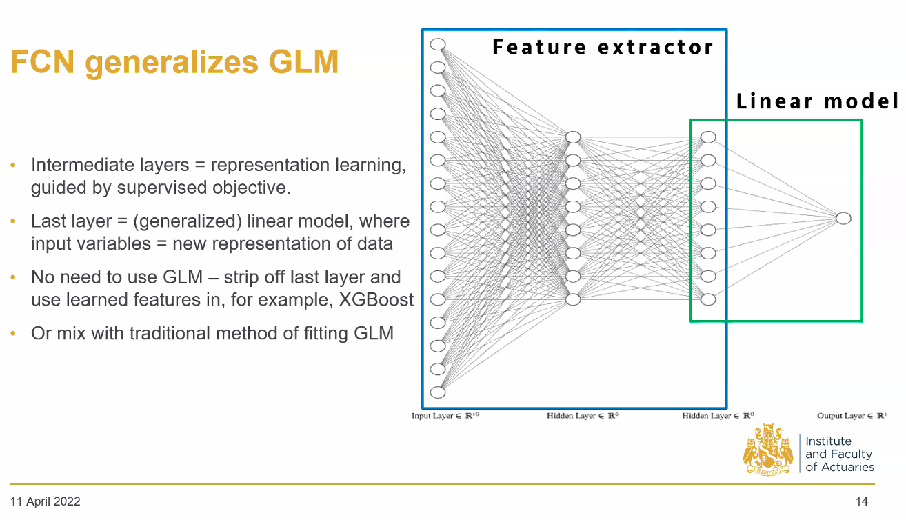
ANN can feed into a GLM

Combining GLM & ANN.

Deep GLM

A GLM has a linear predictor. A deep GLM (Tran et al., 2020) swaps that for a neural network β€” a non-linear mean β€” but keeps the same Gamma loss, so it still predicts a single Gamma distribution.

def gamma_loss(y_true, y_pred):
    return keras.ops.mean(keras.ops.log(y_pred) + y_true / y_pred)

random.seed(1)
inputs = Input(shape=X_train.shape[1:])
x = Dense(64, activation="leaky_relu")(inputs)
x = Dense(64, activation="leaky_relu")(x)
mu = Dense(1, activation="exponential")(x) + 1e-6
deep_glm = Model(inputs, mu)
deep_glm.compile(optimizer="adam", loss=gamma_loss)
deep_glm.fit(X_train, y_train, epochs=100, batch_size=64, verbose=0,
    callbacks=[EarlyStopping(patience=10, restore_best_weights=True)],
    validation_split=0.2);

Combined Actuarial Neural Network

Lecture Outline

  • Introduction

  • Traditional Regression

  • Stochastic Forecasts

  • GLMs and Neural Networks

  • Combined Actuarial Neural Network

  • Mean-Variance Estimation Network

  • Mixture Density Network

  • Distributional Refinement Network

  • Uncertainty and Regularisation

  • Dropout and Ensembles

CANN

The Combined Actuarial Neural Network is an actuarial neural network architecture proposed by Schelldorfer & WΓΌthrich (2019). We summarise the CANN approach as follows:

  • Find coefficients \boldsymbol{\beta} of the GLM with a link function g(\cdot).
  • Find weights \boldsymbol{w} = (\boldsymbol{w}^{(1)}, \dots, \boldsymbol{w}^{(K+1)}) of a neural network s:\mathbb{R}^{p}\to\mathbb{R}.
  • Given a new instance \boldsymbol{x}, we have

\mathbb{E}[Y|\boldsymbol{X}=\boldsymbol{x}] = g^{-1}\Big( \langle\boldsymbol{\beta}, \boldsymbol{x}\rangle + s(\boldsymbol{x};\boldsymbol{w})\Big).

If just a sequential dense network, then

\mathbb{E}[Y|\boldsymbol{X}=\boldsymbol{x}] = g^{-1}\Big( \langle\boldsymbol{\beta}, \boldsymbol{x}\rangle + \Big\langle \boldsymbol{w}^{(K+1)}, \bigl( \boldsymbol{z}^{(K)} \circ \dots \circ \boldsymbol{z}^{(1)}\bigr)(\boldsymbol{x}) \Big\rangle \Big).

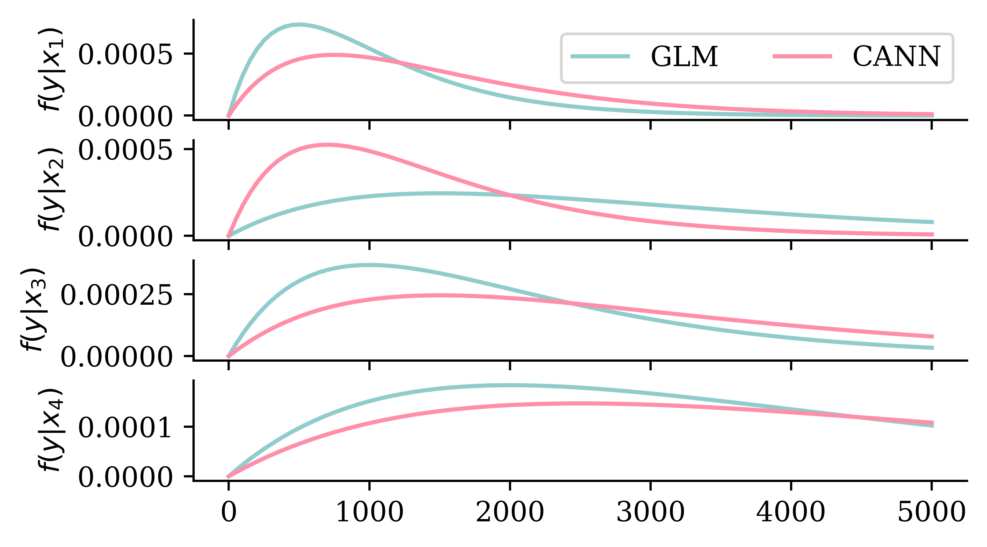
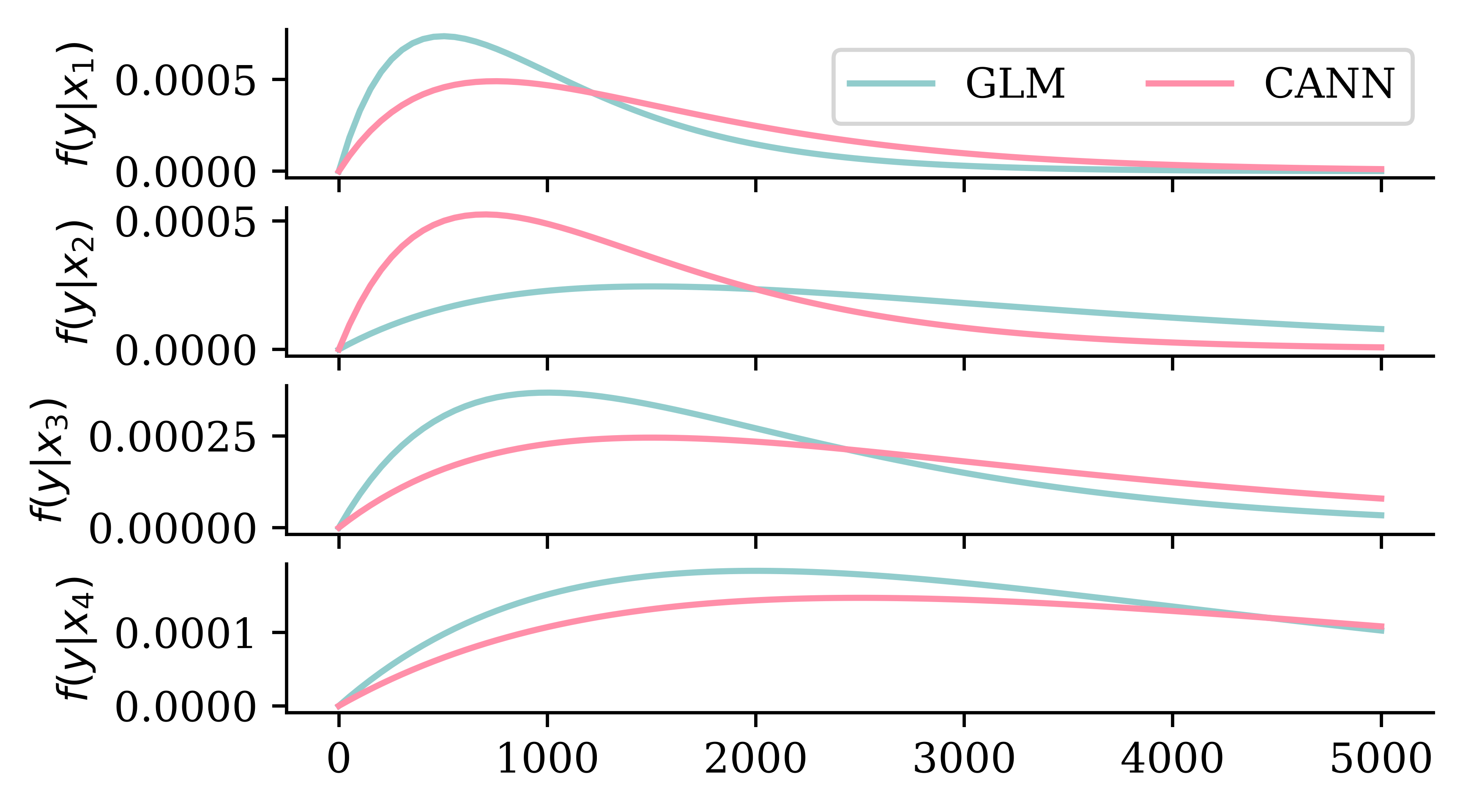
Shifting the predicted distributions

Code
# Ensure reproducibility
random.seed(1)

# Make a 4x1 grid of plots
fig, axes = plt.subplots(4, 1, figsize=(5.0, 3.0), sharex=True)

# Define the x-axis
x_min = 0
x_max = 5000
x_grid = np.linspace(x_min, x_max, 100)

# Plot a few Gamma distribution pdfs with different means.
# Then plot Gamma distributions with shifted means and the same dispersion parameter.
glm_means = [1000, 3000, 2000, 4000]
cann_means = [1500, 1400, 3000, 5000]
for i, ax in enumerate(axes):
    ax.plot(x_grid, stats.gamma.pdf(x_grid, a=2, scale=glm_means[i]/2), label=f'GLM')
    ax.plot(x_grid, stats.gamma.pdf(x_grid, a=2, scale=cann_means[i]/2), label=f'CANN')
    ax.set_ylabel(f'$f(y | x_{i+1})$')
    if i == 0:
        ax.legend(["GLM", "CANN"], loc="upper right", ncol=2)
Architecture
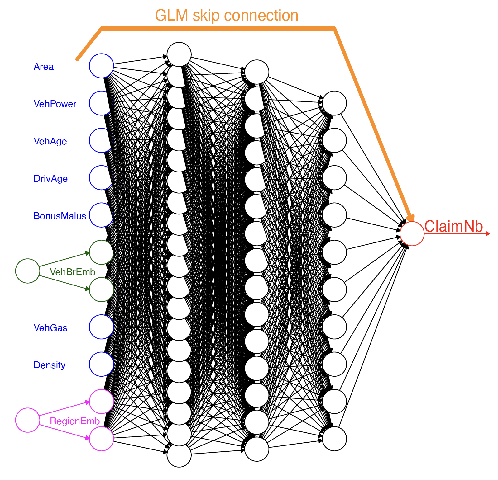
The CANN architecture.

CANN architecture

random.seed(1)
inputs = Input(shape=X_train.shape[1:])

# GLM part (won't be updated during training)
glm_weights = gamma_glm.params.iloc[1:].values.reshape((-1, 1))
glm_bias = gamma_glm.params.iloc[0]
glm_part = Dense(1, activation='linear', trainable=False,
                     kernel_initializer=Constant(glm_weights),
                     bias_initializer=Constant(glm_bias))(inputs)

# Neural network part
x = Dense(64, activation='leaky_relu')(inputs)
nn_part = Dense(1, activation='linear',
                    kernel_initializer="zeros",
                    bias_initializer="zeros")(x)

# Combine GLM and CANN estimates
mu = keras.ops.exp(glm_part + nn_part) + 1e-6
cann = Model(inputs, mu)

Since this CANN predicts Gamma distributions, we reuse the same gamma_loss from the deep GLM.

Training the CANN

cann.compile(optimizer="adam", loss=gamma_loss)
hist = cann.fit(X_train, y_train,
    epochs=100,
    callbacks=[EarlyStopping(patience=10, restore_best_weights=True)],
    verbose=0,
    batch_size=64,
    validation_split=0.2)

Find the dispersion parameter.

mus = cann.predict(X_train, verbose=0).flatten()
residuals = y_train - mus
dof = (len(y_train)-(X_train.shape[1] + 1))
phi_cann = np.sum(residuals**2/mus**2) / dof
print(phi_cann)
64.48475298524968

Mean-Variance Estimation Network

Lecture Outline

  • Introduction

  • Traditional Regression

  • Stochastic Forecasts

  • GLMs and Neural Networks

  • Combined Actuarial Neural Network

  • Mean-Variance Estimation Network

  • Mixture Density Network

  • Distributional Refinement Network

  • Uncertainty and Regularisation

  • Dropout and Ensembles

Generating normal distribution parameters

Our model is

Y \mid \boldsymbol{x} \;\sim\; \mathcal{N}\bigl(\mu(\boldsymbol{x}),\, \sigma^2(\boldsymbol{x})\bigr) .
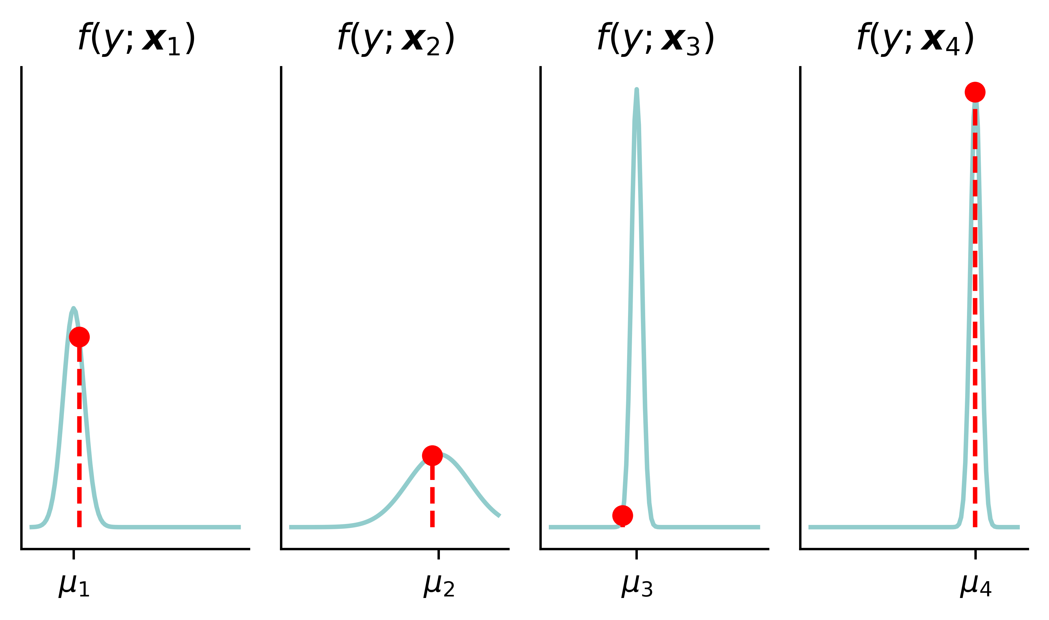
In-class exercise

Make a neural network that models Y \mid \boldsymbol{x} \;\sim\; \mathcal{N}\bigl(\mu(\boldsymbol{x}),\, \sigma^2(\boldsymbol{x})\bigr).

Code
y_pred = np.polyval(coefficients, X_toy[:4])
y_pred[2] *= 1.1
sigma_preds = sigma_toy * np.array([1.0, 3.0, 0.5, 0.5])
fig, axes = plt.subplots(1, 4, figsize=(5.0, 2.0), sharey=True)

x_min = y_pred[:4].min() - 4*sigma_toy
x_max = y_pred[:4].max() + 4*sigma_toy
x_grid = np.linspace(x_min, x_max, 100)

# Plot each normal distribution with different means vertically
for i, ax in enumerate(axes):
    y_grid = stats.norm.pdf(x_grid, y_pred[i], sigma_preds[i])
    ax.plot(x_grid, y_grid)
    ax.plot([y_toy[i], y_toy[i]], [0, stats.norm.pdf(y_toy[i], y_pred[i], sigma_preds[i])], color='red', linestyle='--')
    ax.scatter([y_toy[i]], [stats.norm.pdf(y_toy[i], y_pred[i], sigma_preds[i])], color='red', zorder=10)
    ax.set_title(f'$f(y ; \\boldsymbol{{x}}_{{{i+1}}})$')
    ax.set_xticks([y_pred[i]], labels=[r'$\mu_{' + str(i+1) + r'}$'])
    # ax.set_ylim(0, 0.25)

    # Turn off the y axes
    ax.yaxis.set_visible(False)

plt.tight_layout();
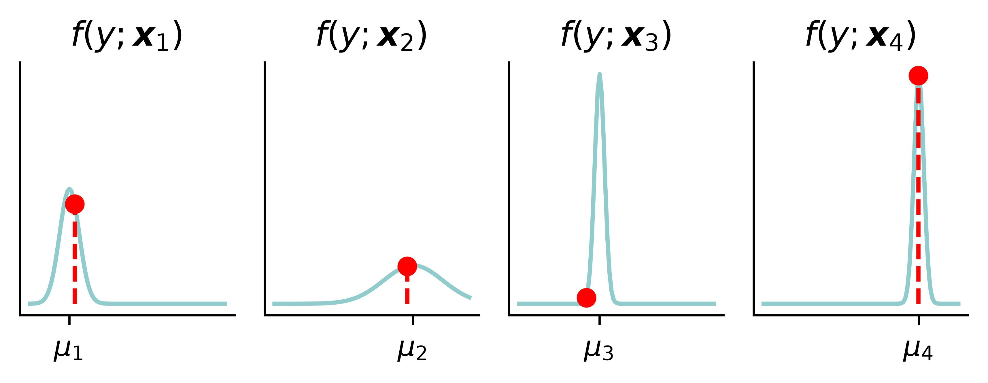
Task: Assume you have X_train and y_train loaded and write the following code, everything up to the model.fit(X_train, y_train) line.

Mixture Density Network

Lecture Outline

  • Introduction

  • Traditional Regression

  • Stochastic Forecasts

  • GLMs and Neural Networks

  • Combined Actuarial Neural Network

  • Mean-Variance Estimation Network

  • Mixture Density Network

  • Distributional Refinement Network

  • Uncertainty and Regularisation

  • Dropout and Ensembles

Mixture density network

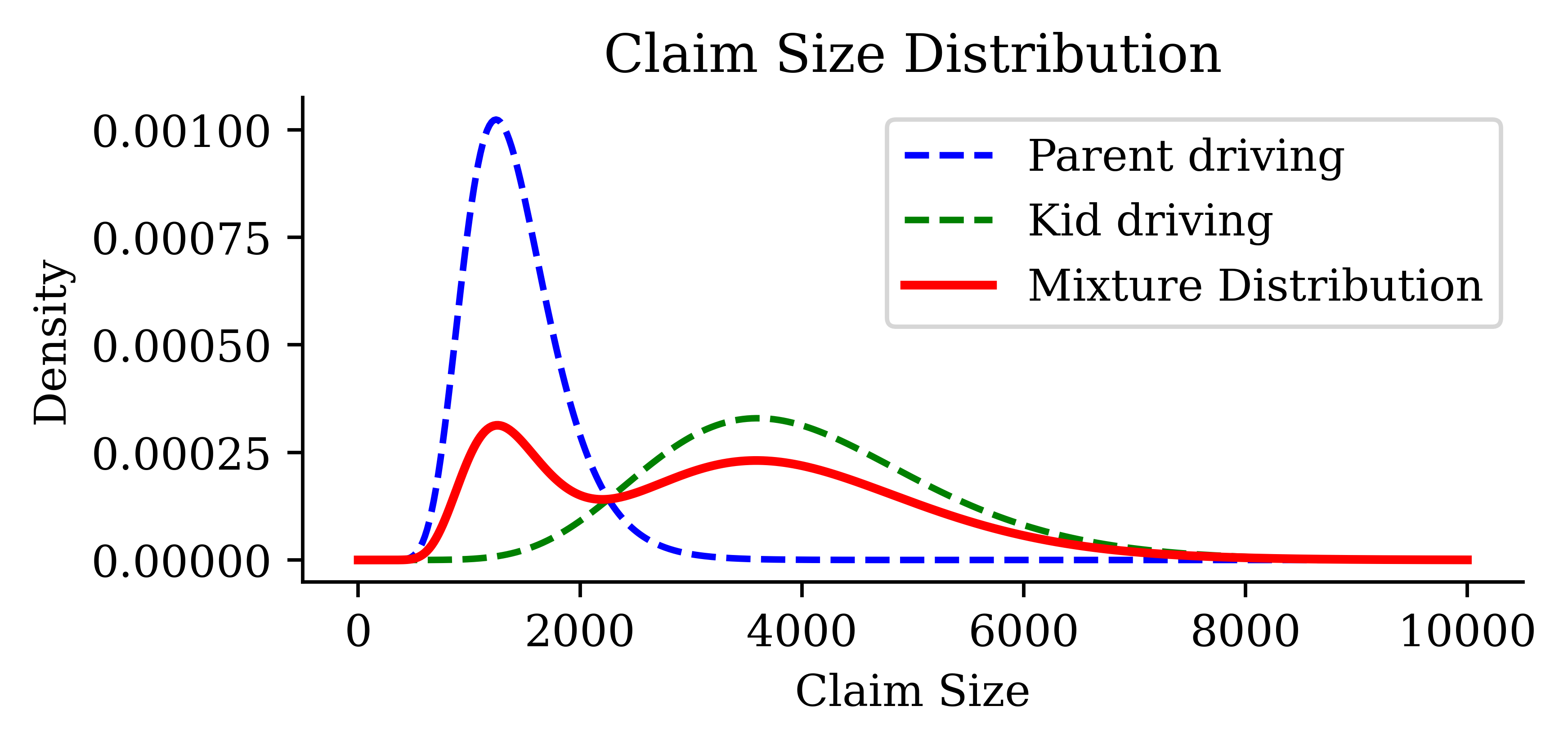
The mean-variance network outputs the parameters of a single normal. But our data may be multimodal, or have some other shape which no single normal or gamma can capture.

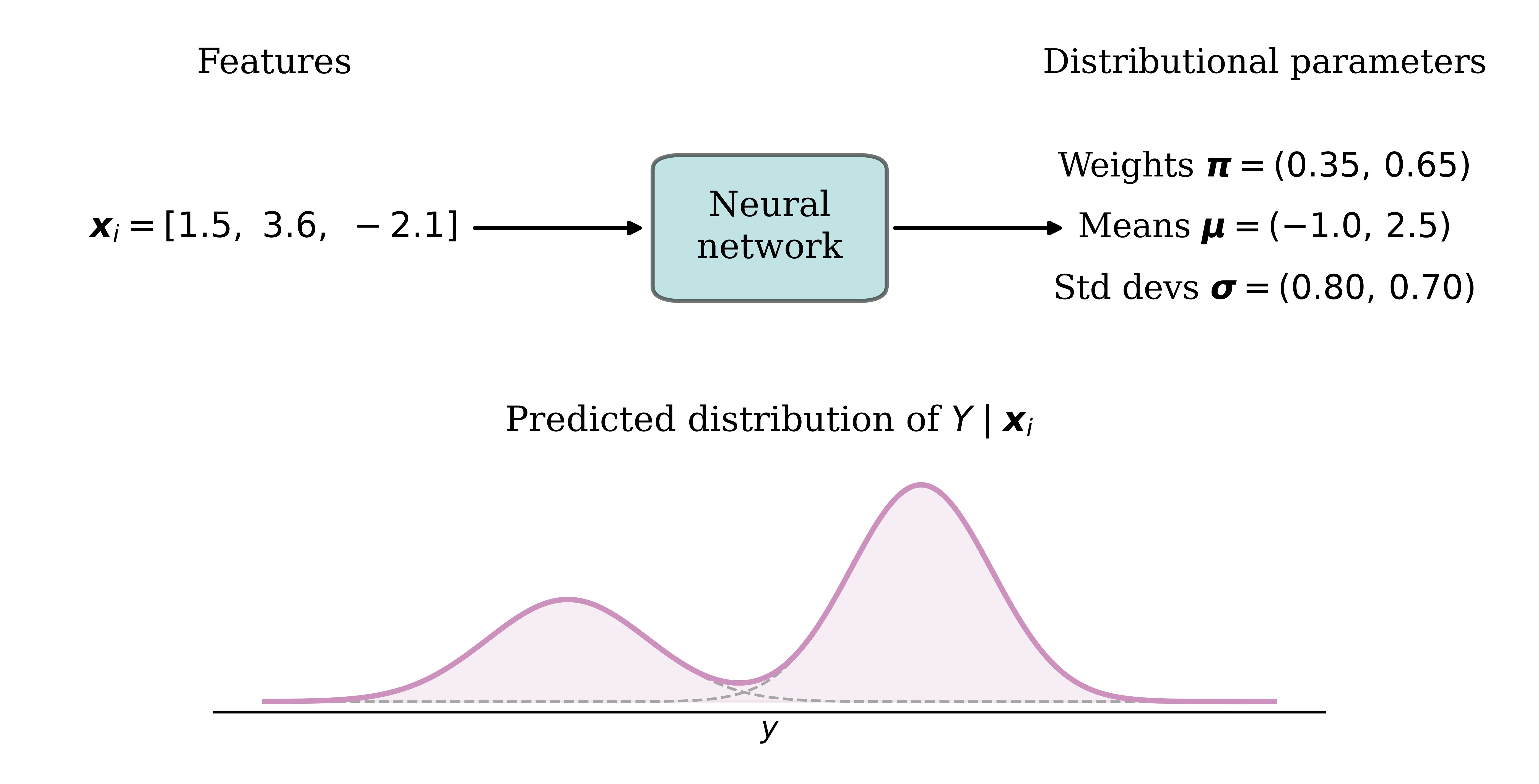
A mixture density network (MDN) operates the same way, except now we model Y \mid \boldsymbol{x} as a mixture of K components. The network outputs the mixing weights \boldsymbol{\pi}(\boldsymbol{x}) and each component’s parameters, giving the density f_{Y|\boldsymbol{X}}(y \mid \boldsymbol{x}) = \sum_{k=1}^{K}\pi_k(\boldsymbol{x})\, f_{k}(y \mid \boldsymbol{x}), \qquad \pi_k(\boldsymbol{x}) \ge 0,\ \ \sum_{k=1}^{K}\pi_k(\boldsymbol{x})=1 . Each component f_k can be any parametric family (normal, gamma, etc.).

A two-component normal MDN

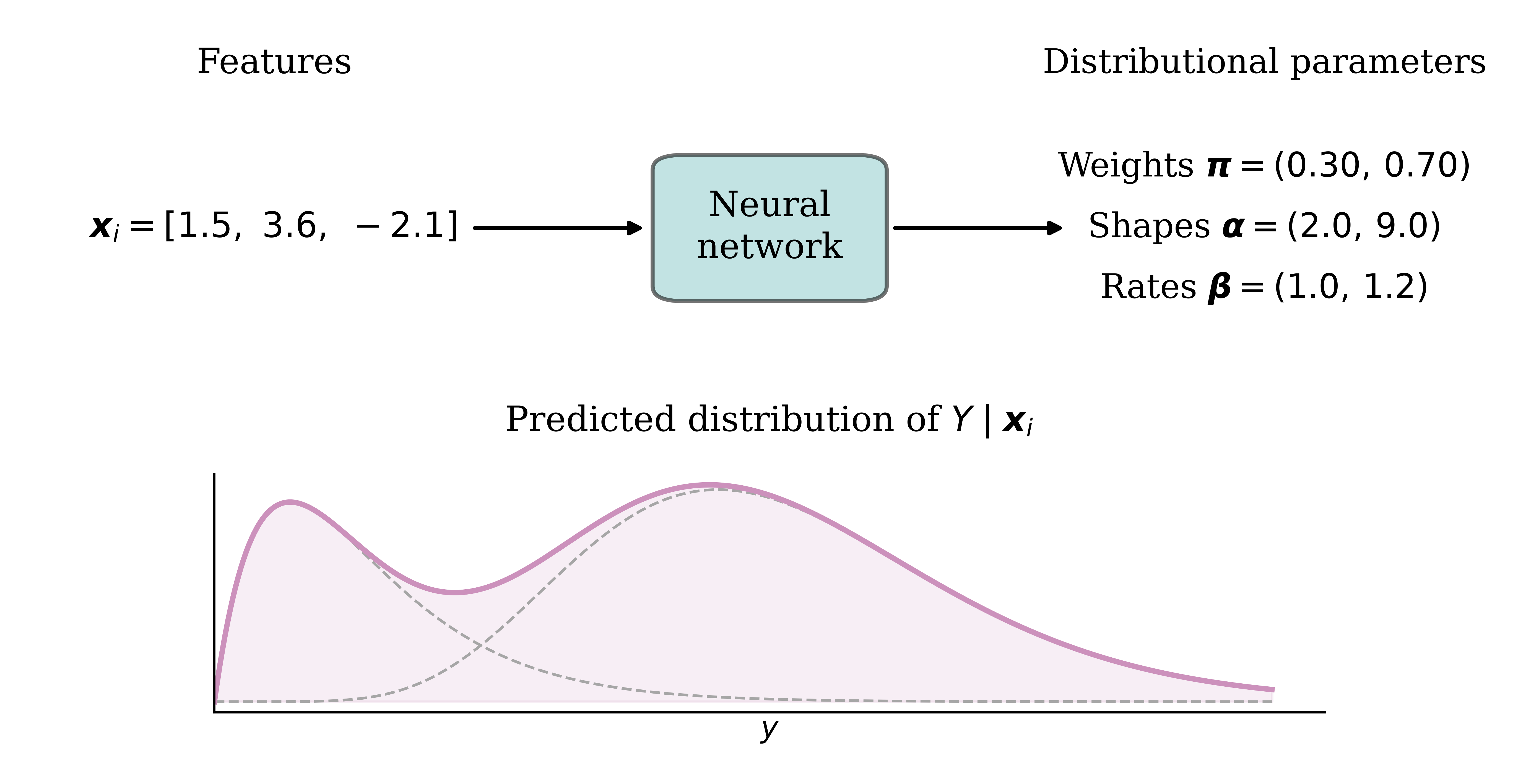
A two-component Gamma mixture

Suppose there are two types of claims:

  • Type I: Y_1|\boldsymbol{X}=\boldsymbol{x}\sim \text{Gamma}(\alpha_1(\boldsymbol{x}), \beta_1(\boldsymbol{x})) and,
  • Type II: Y_2|\boldsymbol{X}=\boldsymbol{x}\sim \text{Gamma}(\alpha_2(\boldsymbol{x}), \beta_2(\boldsymbol{x})).

(Note the new gamma parametrisation.) So the claim amount Y|\boldsymbol{X}=\boldsymbol{x} has density \begin{align*} f_{Y|\boldsymbol{X}}(y|\boldsymbol{x}) &= \pi_1(\boldsymbol{x})\cdot \frac{\beta_1(\boldsymbol{x})^{\alpha_1(\boldsymbol{x})}}{\Gamma(\alpha_1(\boldsymbol{x}))}\mathrm{e}^{-\beta_1(\boldsymbol{x})y}y^{\alpha_1(\boldsymbol{x})-1} \\ &\quad + \pi_2(\boldsymbol{x})\cdot \frac{\beta_2(\boldsymbol{x})^{\alpha_2(\boldsymbol{x})}}{\Gamma(\alpha_2(\boldsymbol{x}))}\mathrm{e}^{-\beta_2(\boldsymbol{x})y}y^{\alpha_2(\boldsymbol{x})-1}, \end{align*} where \pi_1(\boldsymbol{x}) is the probability of a Type I claim. So here the network’s six outputs are the mixing weights, shapes and rates: \text{MDN}(\boldsymbol{x}; \boldsymbol{w}^*) = \bigl( \pi_1, \pi_2,\ \alpha_1, \alpha_2,\ \beta_1, \beta_2 \bigr).

The Gamma MDN

Gamma MDN architecture

The following code implements the gamma MDN from the previous slide.

random.seed(1)

n_components = 2
inputs = Input(shape=X_train.shape[1:])

x = Dense(64, activation="relu")(inputs)
x = Dense(64, activation="relu")(x)

pis = Dense(n_components, activation="softmax")(x)
alphas = Dense(n_components, activation="softplus")(x) + 1e-6
betas = Dense(n_components, activation="softplus")(x) + 1e-6

outputs = Concatenate()([pis, alphas, betas])
gamma_mdn = Model(inputs, outputs)

Loss & training

torch.distributions to the rescue.

def gamma_mixture_nll(y_true, y_pred):
    pis = y_pred[:, :n_components]
    alphas = y_pred[:, n_components:2*n_components]
    betas = y_pred[:, 2*n_components:]
    mixture = MixtureSameFamily(
        mixture_distribution=Categorical(probs=pis),
        component_distribution=Gamma(concentration=alphas, rate=betas))
    return -keras.ops.mean(mixture.log_prob(keras.ops.squeeze(y_true)))

We can now train it like any other Keras model.

gamma_mdn.compile(optimizer="adam", loss=gamma_mixture_nll)
gamma_mdn.fit(X_train, y_train,
    epochs=100,
    callbacks=[EarlyStopping(patience=10, restore_best_weights=True)],
    verbose=0,
    batch_size=64,
    validation_split=0.2)

Distributional Refinement Network

Lecture Outline

  • Introduction

  • Traditional Regression

  • Stochastic Forecasts

  • GLMs and Neural Networks

  • Combined Actuarial Neural Network

  • Mean-Variance Estimation Network

  • Mixture Density Network

  • Distributional Refinement Network

  • Uncertainty and Regularisation

  • Dropout and Ensembles

The DRN architecture

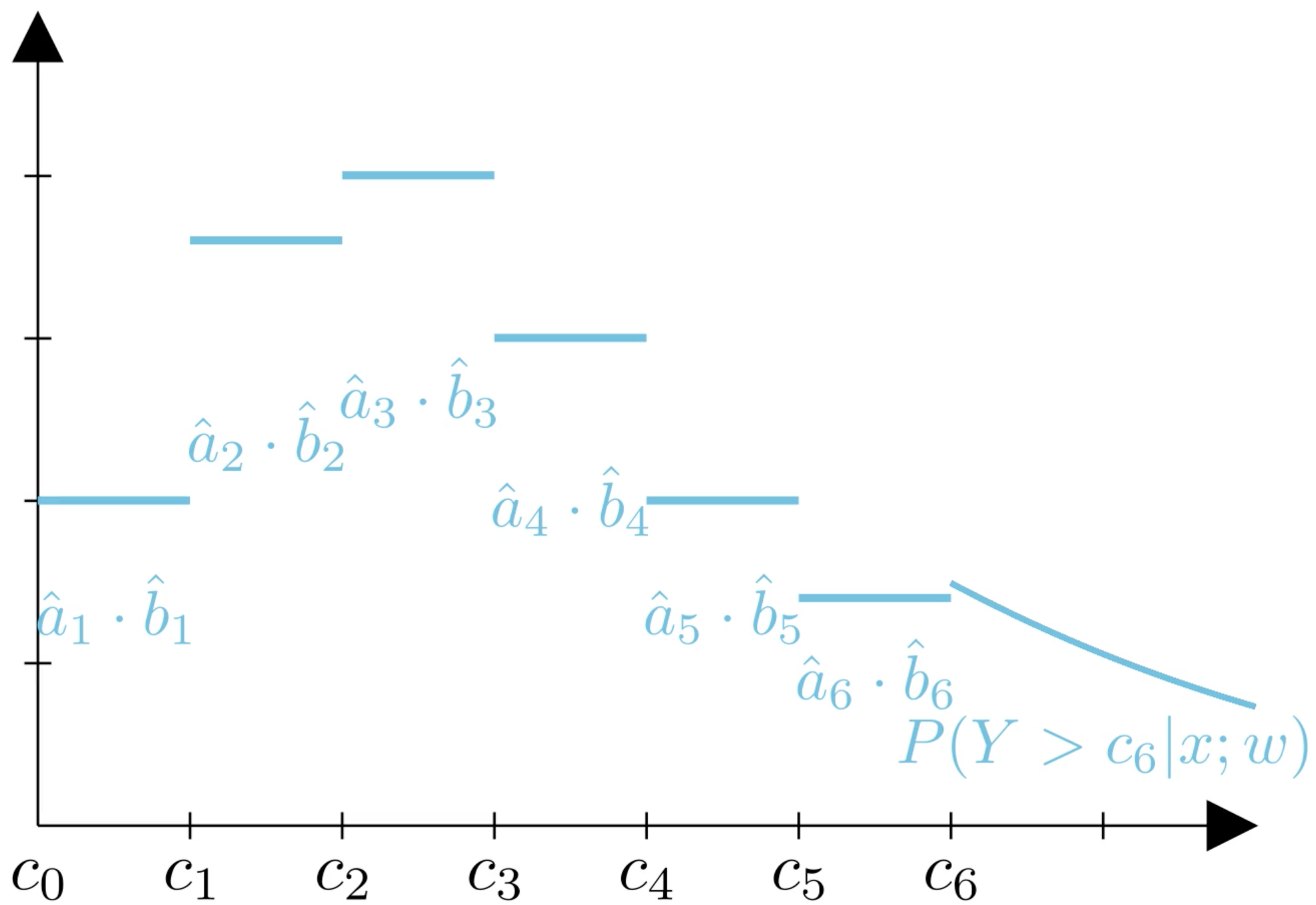
Start from a trusted parametric baseline (e.g. a GLM), then let a neural network make small adjustments to the whole distribution.
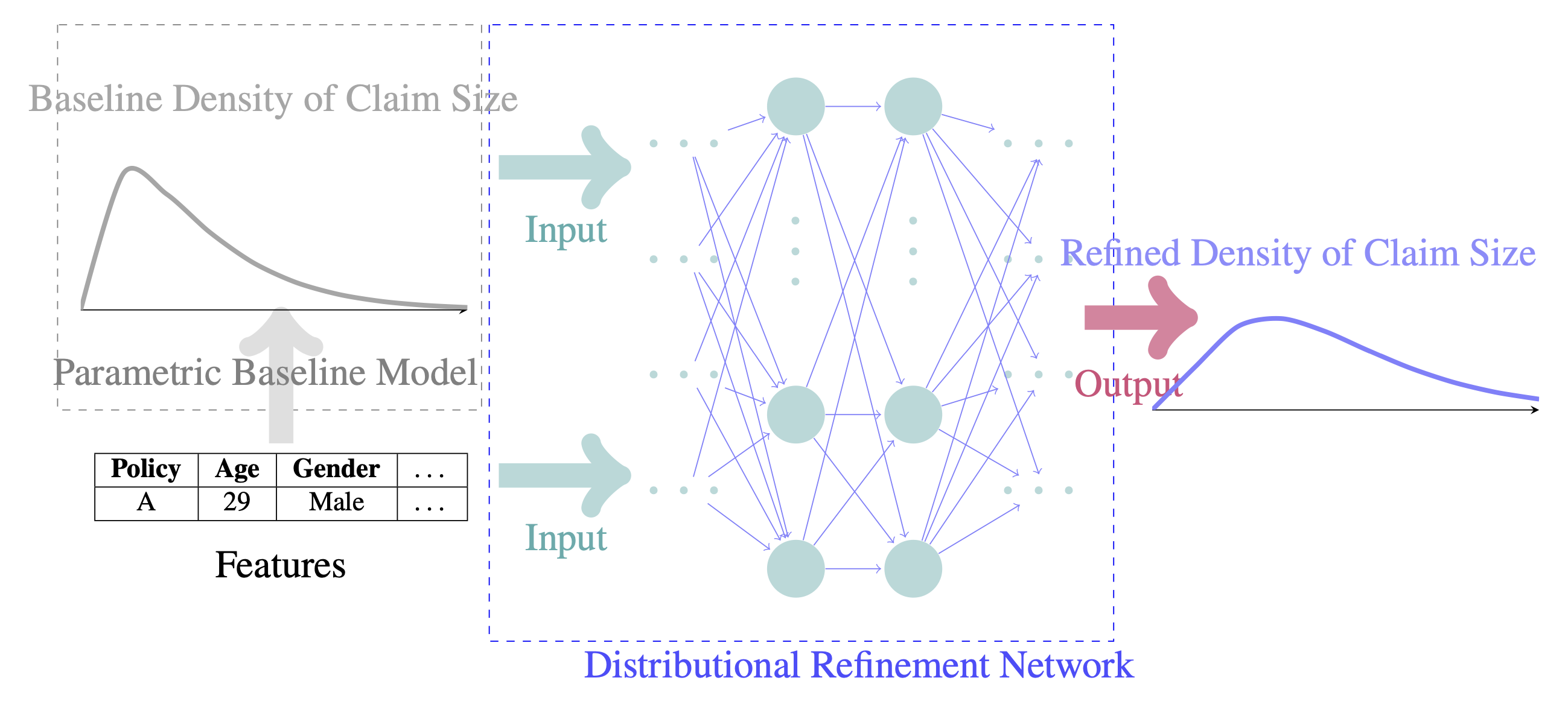
The DRN keeps the baseline’s shape but flexibly refines it using the features.

Refining the distribution

Discretise the baseline into bins, then multiply each bin’s mass by a learned adjustment factor \hat{a}_k.
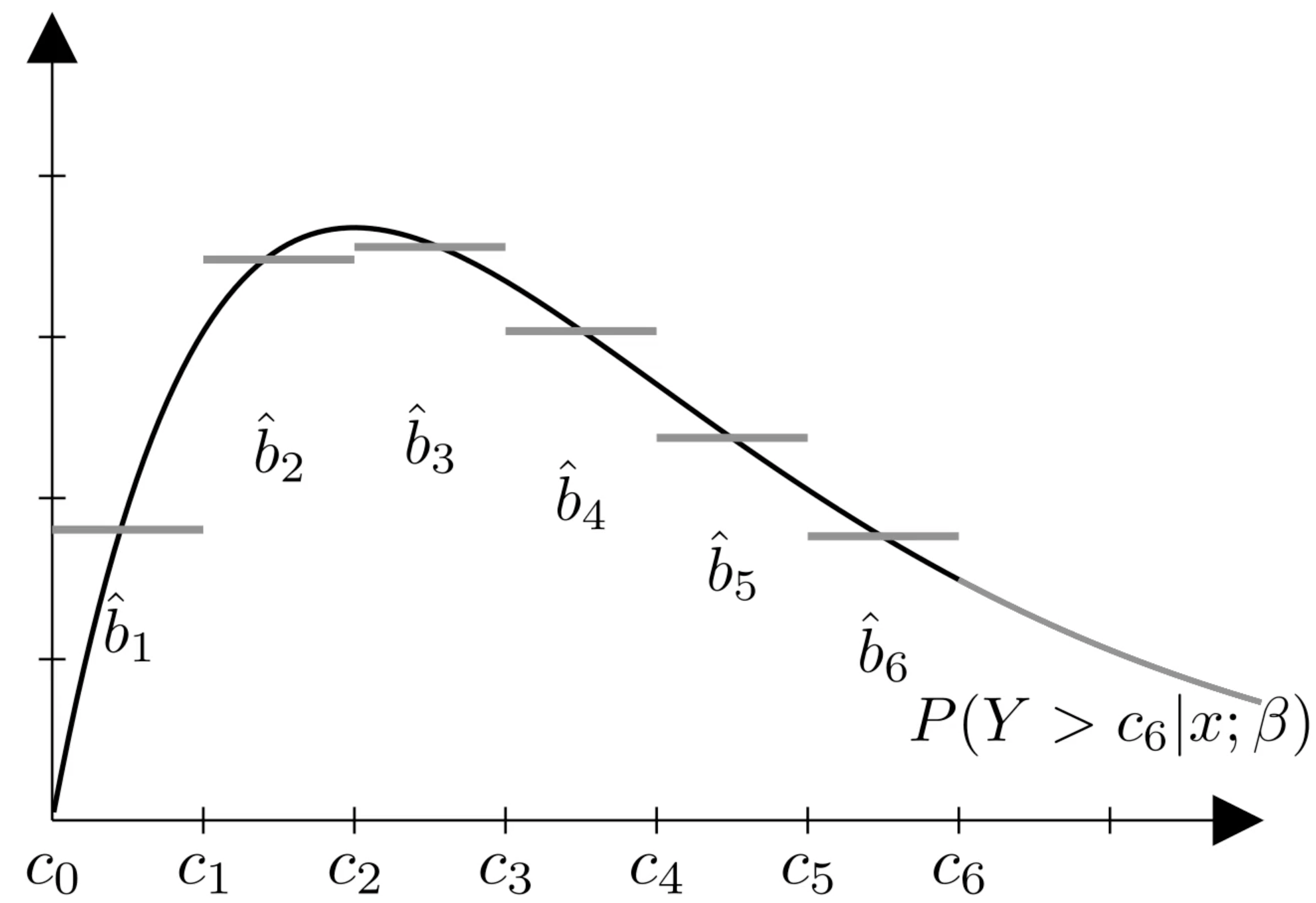
Baseline: discretised masses \hat{b}_k.

Refined: adjusted masses \hat{a}_k \cdot \hat{b}_k.

A penalty keeps the adjustments faithful to the baseline, so the model stays interpretable and trustworthy.

Implemented in the drn package

The drn package fits the DRN architecture along with today’s earlier models:

from drn import GLM, CANN, MDN, DRN, nll

glm  = GLM("gamma").fit(X_train, y_train)
cann = CANN(glm).fit(X_train, y_train)
mdn  = MDN("gamma", num_components=2).fit(X_train, y_train)
drn  = DRN(glm).fit(X_train, y_train)
for name, model in {"GLM": glm, "CANN": cann, "MDN": mdn, "DRN": drn}.items():
    print(f"{name}: {nll(model.predict(X_test), y_test):.2f}")
GLM: 11.02
CANN: 10.27
MDN: 8.78
DRN: 8.32

Uncertainty and Regularisation

Lecture Outline

  • Introduction

  • Traditional Regression

  • Stochastic Forecasts

  • GLMs and Neural Networks

  • Combined Actuarial Neural Network

  • Mean-Variance Estimation Network

  • Mixture Density Network

  • Distributional Refinement Network

  • Uncertainty and Regularisation

  • Dropout and Ensembles

Categories of uncertainty

There are two major categories of uncertainty in statistical or machine learning:

  • Aleatoric uncertainty: the inherent variability associated with the data generating process.
  • Epistemic uncertainty: the lack of knowledge, limited data information, parameter errors and model errors.

Sources of uncertainty

If you decide to predict the claim amount of an individual using a deep learning model, which source(s) of uncertainty are you dealing with?

  1. The inherent variability of the data-generating process \rightarrow aleatoric uncertainty.
  2. Parameter error \rightarrow epistemic uncertainty.
  3. Model error \rightarrow epistemic uncertainty.
  4. Data uncertainty \rightarrow epistemic uncertainty.

Traditional regularisation

Say all the m weights (excluding biases) are in the vector \boldsymbol{\theta}. If we change the loss function to \text{Loss}_{1:n} = \frac{1}{n} \sum_{i=1}^n \text{Loss}_i + \lambda \sum_{j=1}^{m} \left| \theta_j \right|

this would be using L^1 regularisation. A loss like

\text{Loss}_{1:n} = \frac{1}{n} \sum_{i=1}^n \text{Loss}_i + \lambda \sum_{j=1}^{m} \theta_j^2

is called L^2 regularisation.

Regularisation in Keras

Code
features, target = fetch_california_housing(as_frame=True, return_X_y=True)

NUM_FEATURES = len(features.columns)

X_main, X_test, y_main, y_test = train_test_split(
    features, target, test_size=0.2, random_state=1
)
X_train, X_val, y_train, y_val = train_test_split(
    X_main, y_main, test_size=0.25, random_state=1
)

scaler = StandardScaler()
X_train_sc = scaler.fit_transform(X_train)
X_val_sc = scaler.transform(X_val)
X_test_sc = scaler.transform(X_test)
def l1_model(regulariser_strength=0.01):
  random.seed(123)
  model = Sequential([
      Dense(30, activation="leaky_relu",
        kernel_regularizer=L1(regulariser_strength)),
      Dense(1, activation="exponential")
  ])

  model.compile("adam", "mse")
  model.fit(X_train_sc, y_train, epochs=4, verbose=0)
  return model

def l2_model(regulariser_strength=0.01):
  random.seed(123)
  model = Sequential([
      Dense(30, activation="leaky_relu",
        kernel_regularizer=L2(regulariser_strength)),
      Dense(1, activation="exponential")
  ])

  model.compile("adam", "mse")
  model.fit(X_train_sc, y_train, epochs=10, verbose=0)
  return model

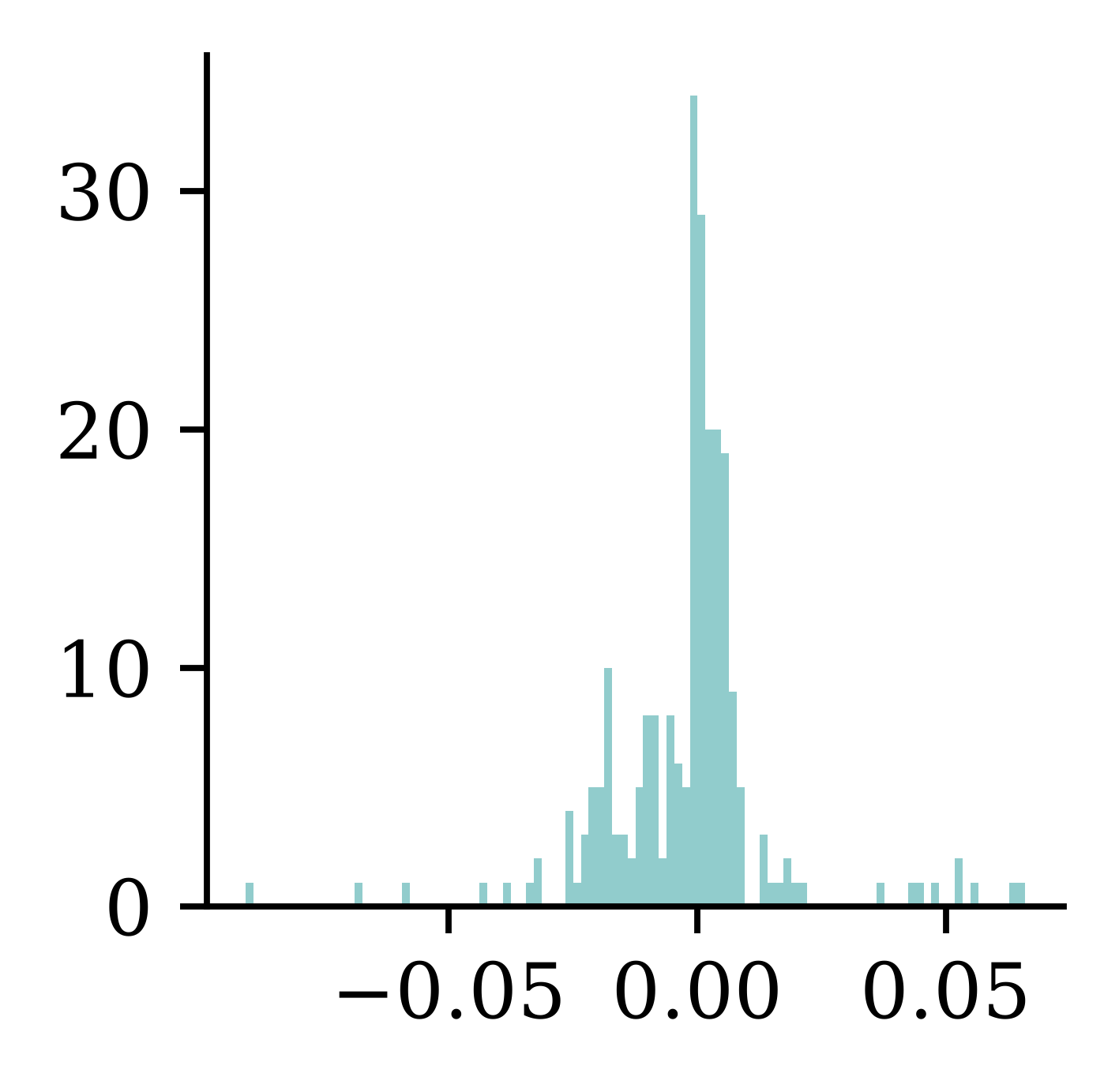
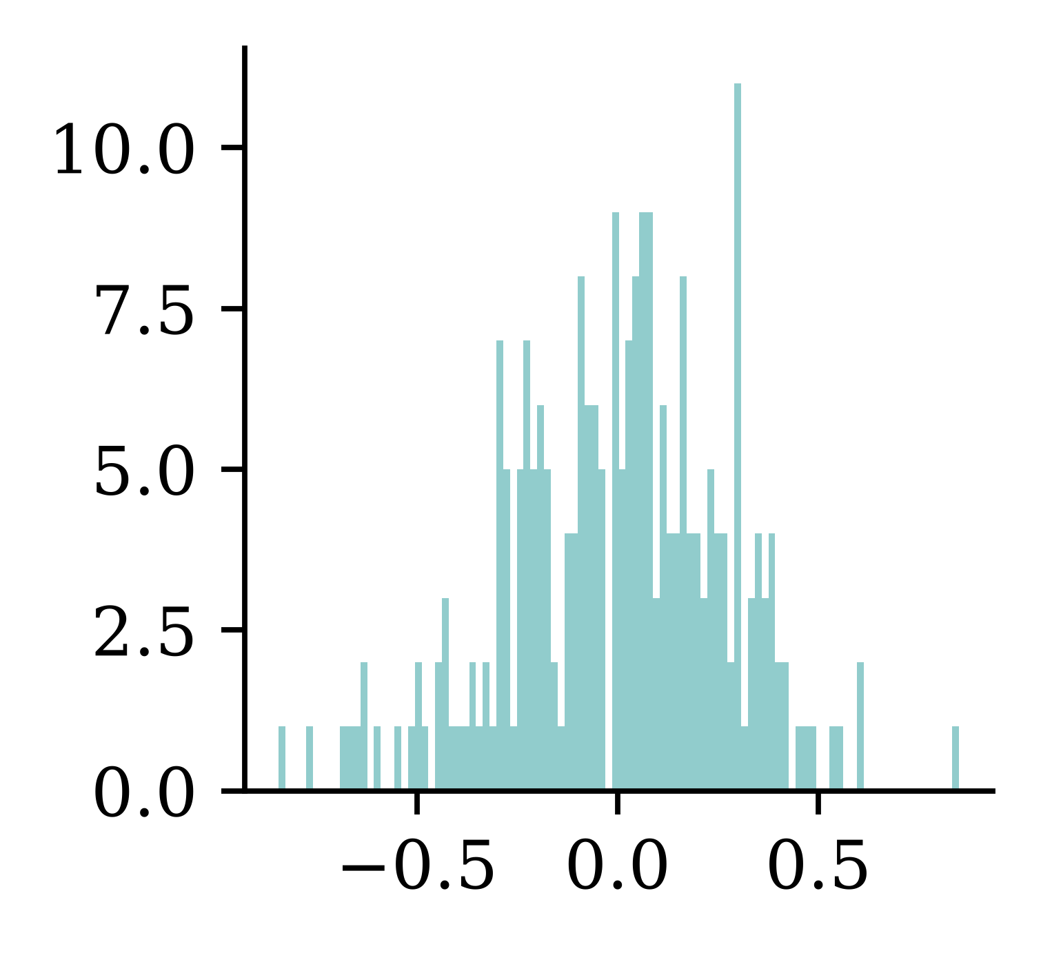
Weights before & after L^2

model = l2_model(0.0)
weights = model.layers[0].get_weights()[0].flatten()
print(f"Number of weights almost 0: {np.sum(np.abs(weights) < 1e-5)}")
plt.hist(weights, bins=100);
Number of weights almost 0: 0

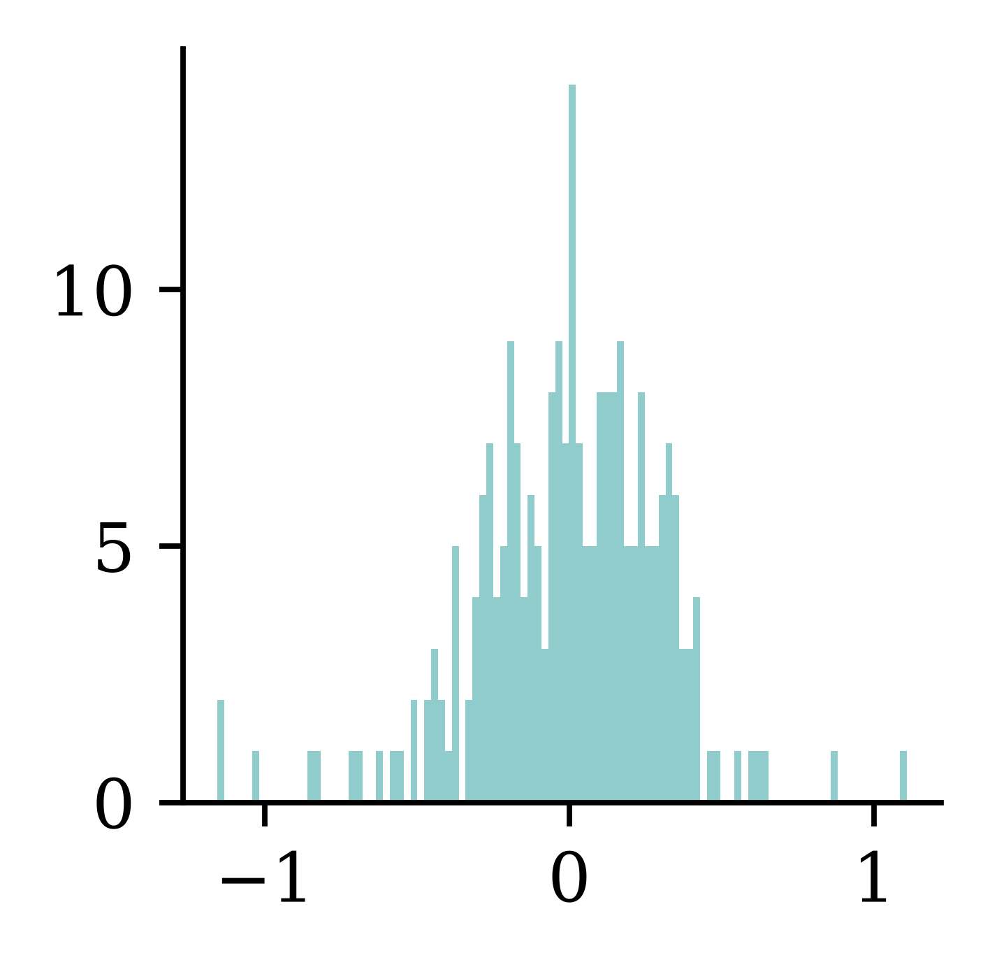
model = l2_model(1.0)
weights = model.layers[0].get_weights()[0].flatten()
print(f"Number of weights almost 0: {np.sum(np.abs(weights) < 1e-5)}")
plt.hist(weights, bins=100);
Number of weights almost 0: 6

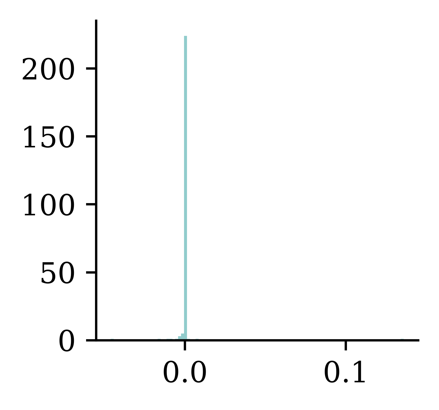
Weights before & after L^1

model = l1_model(0.0)
weights = model.layers[0].get_weights()[0].flatten()
print(f"Number of weights almost 0: {np.sum(np.abs(weights) < 1e-5)}")
plt.hist(weights, bins=100);
Number of weights almost 0: 0

model = l1_model(1.0)
weights = model.layers[0].get_weights()[0].flatten()
print(f"Number of weights almost 0: {np.sum(np.abs(weights) < 1e-5)}")
plt.hist(weights, bins=100);
Number of weights almost 0: 12

Early-stopping regularisation

A very different way to regularize iterative learning algorithms such as gradient descent is to stop training as soon as the validation error reaches a minimum. This is called early stopping… It is such a simple and efficient regularization technique that Geoffrey Hinton called it a β€œbeautiful free lunch”.

Alternatively, you can try building a model with slightly more layers and neurons than you actually need, then use early stopping and other regularization techniques to prevent it from overfitting too much. Vincent Vanhoucke, a scientist at Google, has dubbed this the β€œstretch pants” approach: instead of wasting time looking for pants that perfectly match your size, just use large stretch pants that will shrink down to the right size.

Dropout and Ensembles

Lecture Outline

  • Introduction

  • Traditional Regression

  • Stochastic Forecasts

  • GLMs and Neural Networks

  • Combined Actuarial Neural Network

  • Mean-Variance Estimation Network

  • Mixture Density Network

  • Distributional Refinement Network

  • Uncertainty and Regularisation

  • Dropout and Ensembles

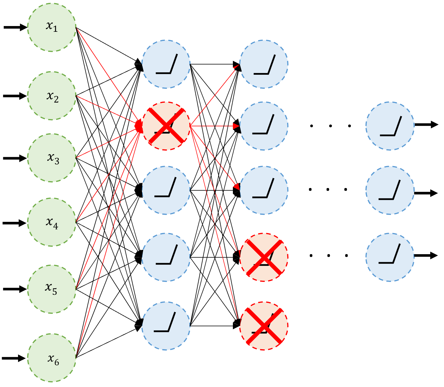
Dropout

An example of neurons dropped during training.

Dropout quote

It’s surprising at first that this destructive technique works at all. Would a company perform better if its employees were told to toss a coin every morning to decide whether or not to go to work? Well, who knows; perhaps it would! The company would be forced to adapt its organization; it could not rely on any single person to work the coffee machine or perform any other critical tasks, so this expertise would have to be spread across several people. Employees would have to learn to cooperate with many of their coworkers, not just a handful of them. The company would become much more resilient. If one person quit, it wouldn’t make much of a difference. It’s unclear whether this idea would actually work for companies, but it certainly does for neural networks. Neurons trained with dropout cannot co-adapt with their neighboring neurons; they have to be as useful as possible on their own. They also cannot rely excessively on just a few input neurons; they must pay attention to each of their input neurons. They end up being less sensitive to slight changes in the inputs. In the end, you get a more robust network that generalizes better.

Dropout

Dropout is just another layer in Keras.

random.seed(2);

model = Sequential([
    Dense(30, activation="leaky_relu"),
    Dropout(0.2),
    Dense(30, activation="leaky_relu"),
    Dropout(0.2),
    Dense(1, activation="exponential")
])

model.compile("adam", "mse")
model.fit(X_train_sc, y_train, epochs=4, verbose=0);

Dropout after training

Making predictions is the same as any other model:

model.predict(X_train_sc.head(3),
                  verbose=0)
array([[1.73],
       [0.74],
       [1.56]], dtype=float32)
model.predict(X_train_sc.head(3),
                  verbose=0)
array([[1.73],
       [0.74],
       [1.56]], dtype=float32)

We can make the model think it is still training:

keras.ops.convert_to_numpy(
    model(X_train_sc.head(3), training=True))
array([[2.08],
       [0.85],
       [1.43]], dtype=float32)
keras.ops.convert_to_numpy(
    model(X_train_sc.head(3), training=True))
array([[1.71],
       [0.6 ],
       [1.51]], dtype=float32)

By setting the training=True, we can let dropout happen during prediction stage as well. This will change predictions for the same output differently. This is known as the Monte Carlo dropout and can be used to generate a distribution of predictions.

Ensembles

Combine many models to get better predictions.

Deep Ensembles

Train M neural networks with different random initial weights independently (even in parallel).

def build_model(seed):
    random.seed(seed)
    model = Sequential([
        Dense(30, activation="leaky_relu"),
        Dense(1, activation="exponential")
    ])                                                                      
    model.compile("adam", "mse")                                           

    es = EarlyStopping(restore_best_weights=True, patience=5)
    model.fit(X_train_sc, y_train, epochs=1_000,
        callbacks=[es], validation_data=(X_val_sc, y_val), verbose=False)
    return model
M = 3
seeds = range(M)
models = []
for seed in seeds:
    models.append(build_model(seed))

Deep Ensembles II

Say the trained weights for the NNs are \boldsymbol{w}^{(1)}, \ldots, \boldsymbol{w}^{(M)}, then we get predictions \bigl\{ \hat{y}(\boldsymbol{x}; \boldsymbol{w}^{(m)}) \bigr\}_{m=1}^{M}

y_preds = []
for model in models:
    y_preds.append(model.predict(X_test_sc, verbose=0))

y_preds = np.array(y_preds)
y_preds
array([[[3.36],
        [0.79],
        [2.33],
        ...,
        [2.42],
        [2.43],
        [1.09]],

       [[1.66],
        [1.13],
        [1.72],
        ...,
        [1.91],
        [1.94],
        [2.34]],

       [[2.94],
        [0.92],
        [2.41],
        ...,
        [2.26],
        [2.54],
        [1.31]]], shape=(3, 4128, 1), dtype=float32)

Package Versions

from watermark import watermark
print(watermark(python=True, packages="keras,matplotlib,numpy,pandas,seaborn,scipy,torch,drn"))
Python implementation: CPython
Python version       : 3.14.5
IPython version      : 9.15.0

keras     : 3.15.0
matplotlib: 3.11.0
numpy     : 2.5.0
pandas    : 3.0.3
seaborn   : 0.13.2
scipy     : 1.18.0
torch     : 2.12.1
drn       : 1.0.0

Glossary

  • aleatoric and epistemic uncertainty
  • Combined Actuarial Neural Network
  • Deep GLM
  • Deep Ensembles
  • distributional forecasts
  • Distributional Refinement Network
  • dropout
  • Mixture Density Network
  • mixture distribution
  • Monte Carlo dropout

References

Al-Mudafer, M. T., Avanzi, B., Taylor, G., & Wong, B. (2022). Stochastic loss reserving with mixture density neural networks. Insurance: Mathematics and Economics, 105, 144–174.
Avanzi, B., Dong, E. T., Laub, P. J., & Wong, B. (2026). Distributional refinement network: Distributional forecasting via deep learning. Insurance: Mathematics and Economics, 128, 103246.
Bishop, C. M. (1994). Mixture density networks.
Delong, Ł., Lindholm, M., & WΓΌthrich, M. V. (2021). Gamma mixture density networks and their application to modelling insurance claim amounts. Insurance: Mathematics and Economics, 101, 240–261.
Guo, C., Pleiss, G., Sun, Y., & Weinberger, K. Q. (2017). On calibration of modern neural networks. International Conference on Machine Learning, 1321–1330.
Nix, D. A., & Weigend, A. S. (1994). Estimating the mean and variance of the target probability distribution. Proceedings of 1994 Ieee International Conference on Neural Networks (ICNN’94), 1, 55–60.
Schelldorfer, J., & WΓΌthrich, M. V. (2019). Nesting classical actuarial models into neural networks. Available at SSRN 3320525.
Tran, M.-N., Nguyen, N., Nott, D., & Kohn, R. (2020). Bayesian deep net GLM and GLMM. Journal of Computational and Graphical Statistics, 29(1), 97–113.