Computer Vision

ACTL3143 & ACTL5111 Deep Learning for Actuaries

Author

Patrick Laub

Introduction

What is Computer Vision?

“Little by little, we’re giving sight to the machines. First, we teach them to see. Then, they help us to see better.”

— Fei-Fei Li, creator of ImageNet

Getting computers to extract meaning from images and video — and act on what they see.

Image classification — one label per image (benign vs malignant lesion, pass/fail parts).
Object detection — locate and label many objects at once (pedestrians and traffic lights for a self-driving car).
Image segmentation — label every pixel (outlining a tumour in a scan).
Facial recognition — verify or identify a person (phone unlock, passport gates).

Computer vision for actuaries

Claims automation — estimate motor repair costs from photos of the damage.
Property underwriting — score roof condition and bushfire exposure from aerial imagery.
Health & life — predict cardiovascular risk factors from retinal scans.
Fraud detection — flag reused, stock, or AI-altered claim images.

For an actuary the practical upshot is less about any individual architecture and more about transfer learning: a CNN trained on millions of images can be downloaded and reused on your own (much smaller) dataset.

Facial analytics and life insurance

Since November 2015, created AI to predict mortality from photos.

Imports needed for these demos

import random
from pathlib import Path

import matplotlib.pyplot as plt
import matplotlib.font_manager as fm
from matplotlib.image import imread
from matplotlib.pyplot import imshow
import numpy as np
import pandas as pd
from PIL import Image

import keras
from keras.models import Sequential, Model
from keras.layers import (Dense, Input, Rescaling, Flatten,
    Conv2D, MaxPooling2D, GlobalAveragePooling2D)
from keras.callbacks import EarlyStopping
from keras.utils import plot_model

from sklearn.model_selection import train_test_split
from sklearn.preprocessing import StandardScaler

from directory_tree import DisplayTree
import optuna

For PIL, you’ll need to pip install Pillow.

Shapes of data

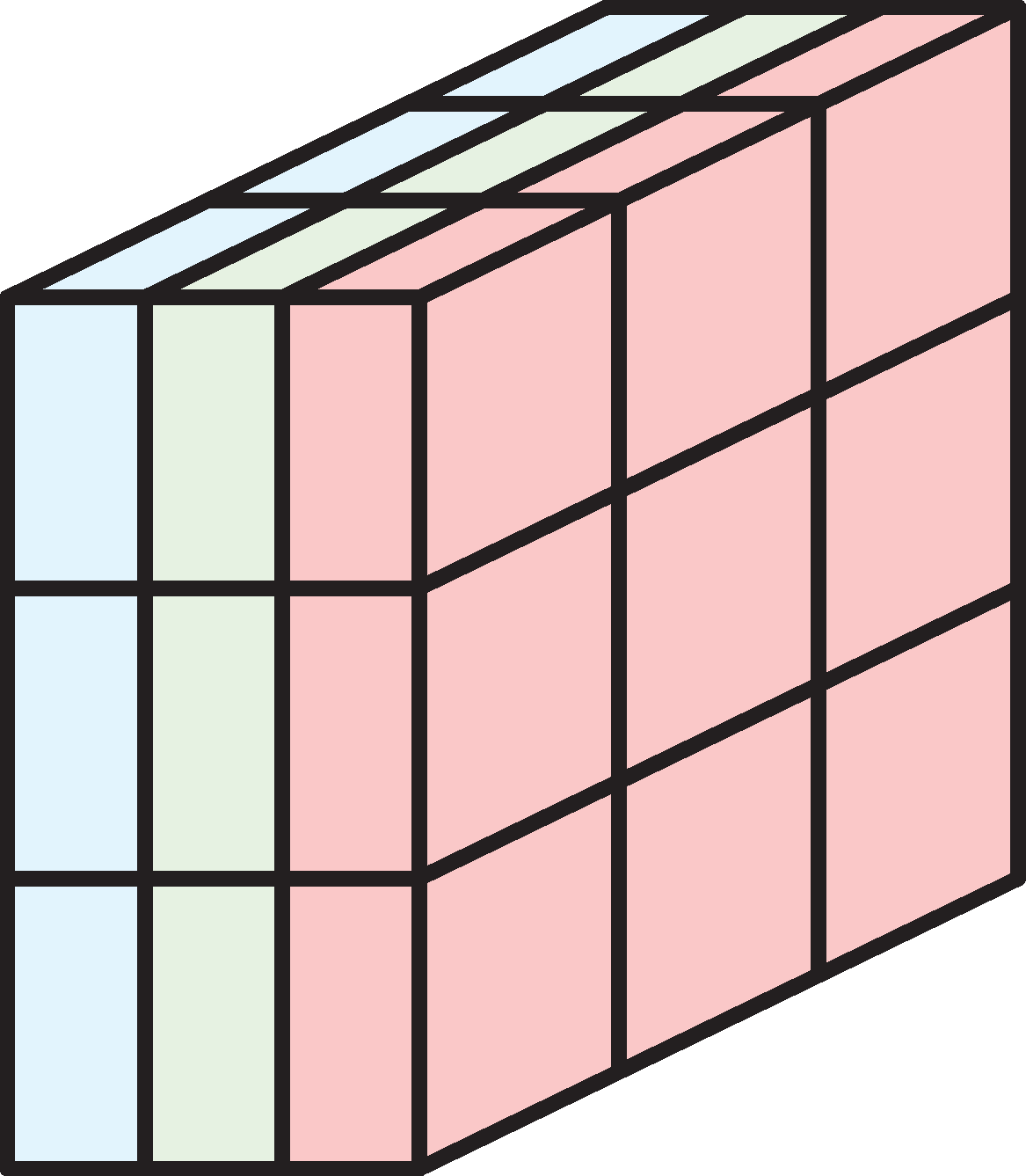
Special attention to the shapes of data is important in CNN architectures, because CNNs have special types of layers (e.g. convolution and pooling) which require explicit specifications of array dimensions.

Illustration of tensors of different rank.

Shapes of photos

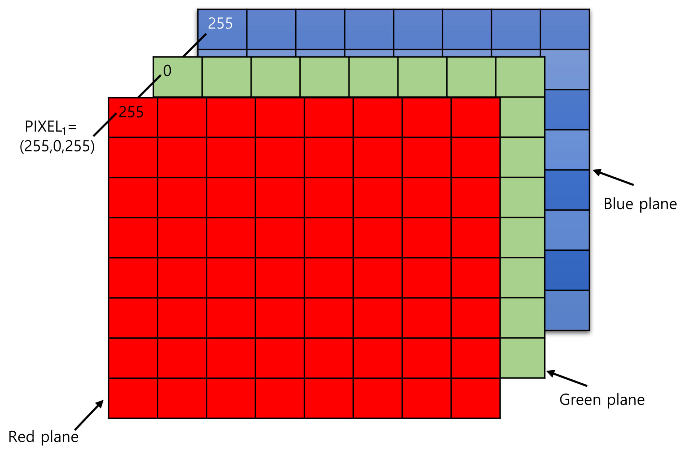
A colour photo is stored as a rank 3 tensor: height × width × colour channels. The first two axes locate a pixel (its row and column), and the third holds that pixel’s three colour intensities (red, green, and blue).

How the computer sees them

img1 = imread('images/pu.gif'); img2 = imread('images/pl.gif')
img3 = imread('images/pr.gif'); img4 = imread('images/pg.bmp')
f"Shapes are: {img1.shape}, {img2.shape}, {img3.shape}, {img4.shape}."

'Shapes are: (16, 16, 3), (16, 16, 3), (16, 16, 3), (16, 16, 3).'

print(img1)

[[[  0   0   0]
  [  0   0   0]
  [  0   0   0]
  [  0   0   0]
  [  0   0   0]
  [  0   0   0]
  [  0   0   0]
  [  0   0   0]
  [  0   0   0]
  [  0   0   0]
  [  0   0   0]
  [  0   0   0]
  [  0   0   0]
  [  0   0   0]
  [  0   0   0]
  [  0   0   0]]

 [[  0   0   0]
  [  0   0   0]
  [  0   0   0]
  [  0   0   0]
  [  0   0   0]
  [  0   0   0]
  [  0   0   0]
  [  0   0   0]
  [  0   0   0]
  [  0   0   0]
  [  0   0   0]
  [  0   0   0]
  [  0   0   0]
  [  0   0   0]
  [  0   0   0]
  [  0   0   0]]

 [[  0   0   0]
  [  0   0   0]
  [  0   0   0]
  [255 255   0]
  [  0   0   0]
  [  0   0   0]
  [  0   0   0]
  [  0   0   0]
  [  0   0   0]
  [  0   0   0]
  [  0   0   0]
  [  0   0   0]
  [255 255   0]
  [  0   0   0]
  [  0   0   0]
  [  0   0   0]]

 [[  0   0   0]
  [  0   0   0]
  [255 255   0]
  [255 255   0]
  [255 255   0]
  [  0   0   0]
  [  0   0   0]
  [  0   0   0]
  [  0   0   0]
  [  0   0   0]
  [  0   0   0]
  [255 255   0]
  [255 255   0]
  [255 255   0]
  [  0   0   0]
  [  0   0   0]]

 [[  0   0   0]
  [255 255   0]
  [255 255   0]
  [255 255   0]
  [255 255   0]
  [  0   0   0]
  [  0   0   0]
  [  0   0   0]
  [  0   0   0]
  [  0   0   0]
  [  0   0   0]
  [255 255   0]
  [255 255   0]
  [255 255   0]
  [255 255   0]
  [  0   0   0]]

 [[  0   0   0]
  [255 255   0]
  [255 255   0]
  [255 255   0]
  [255 255   0]
  [255 255   0]
  [  0   0   0]
  [  0   0   0]
  [  0   0   0]
  [  0   0   0]
  [255 255   0]
  [255 255   0]
  [255 255   0]
  [255 255   0]
  [255 255   0]
  [  0   0   0]]

 [[255 255   0]
  [255 255   0]
  [255 255   0]
  [255 255   0]
  [255 255   0]
  [255 255   0]
  [  0   0   0]
  [  0   0   0]
  [  0   0   0]
  [  0   0   0]
  [255 255   0]
  [255 255   0]
  [255 255   0]
  [255 255   0]
  [255 255   0]
  [255 255   0]]

 [[255 255   0]
  [255 255   0]
  [255 255   0]
  [255 255   0]
  [255 255   0]
  [255 255   0]
  [255 255   0]
  [  0   0   0]
  [  0   0   0]
  [255 255   0]
  [255 255   0]
  [255 255   0]
  [  0   0   0]
  [255 255   0]
  [255 255   0]
  [255 255   0]]

 [[255 255   0]
  [255 255   0]
  [255 255   0]
  [255 255   0]
  [255 255   0]
  [255 255   0]
  [255 255   0]
  [  0   0   0]
  [  0   0   0]
  [255 255   0]
  [255 255   0]
  [255 255   0]
  [255 255   0]
  [255 255   0]
  [255 255   0]
  [255 255   0]]

 [[255 255   0]
  [255 255   0]
  [255 255   0]
  [255 255   0]
  [255 255   0]
  [255 255   0]
  [255 255   0]
  [255 255   0]
  [255 255   0]
  [255 255   0]
  [255 255   0]
  [255 255   0]
  [255 255   0]
  [255 255   0]
  [255 255   0]
  [255 255   0]]

 [[  0   0   0]
  [255 255   0]
  [255 255   0]
  [255 255   0]
  [255 255   0]
  [255 255   0]
  [255 255   0]
  [255 255   0]
  [255 255   0]
  [255 255   0]
  [255 255   0]
  [255 255   0]
  [255 255   0]
  [255 255   0]
  [255 255   0]
  [  0   0   0]]

 [[  0   0   0]
  [255 255   0]
  [255 255   0]
  [255 255   0]
  [255 255   0]
  [255 255   0]
  [255 255   0]
  [255 255   0]
  [255 255   0]
  [255 255   0]
  [255 255   0]
  [255 255   0]
  [255 255   0]
  [255 255   0]
  [255 255   0]
  [  0   0   0]]

 [[  0   0   0]
  [  0   0   0]
  [255 255   0]
  [255 255   0]
  [255 255   0]
  [255 255   0]
  [255 255   0]
  [255 255   0]
  [255 255   0]
  [255 255   0]
  [255 255   0]
  [255 255   0]
  [255 255   0]
  [255 255   0]
  [  0   0   0]
  [  0   0   0]]

 [[  0   0   0]
  [  0   0   0]
  [  0   0   0]
  [255 255   0]
  [255 255   0]
  [255 255   0]
  [255 255   0]
  [255 255   0]
  [255 255   0]
  [255 255   0]
  [255 255   0]
  [255 255   0]
  [255 255   0]
  [  0   0   0]
  [  0   0   0]
  [  0   0   0]]

 [[  0   0   0]
  [  0   0   0]
  [  0   0   0]
  [  0   0   0]
  [255 255   0]
  [255 255   0]
  [255 255   0]
  [255 255   0]
  [255 255   0]
  [255 255   0]
  [255 255   0]
  [255 255   0]
  [  0   0   0]
  [  0   0   0]
  [  0   0   0]
  [  0   0   0]]

 [[  0   0   0]
  [  0   0   0]
  [  0   0   0]
  [  0   0   0]
  [  0   0   0]
  [  0   0   0]
  [255 255   0]
  [255 255   0]
  [255 255   0]
  [255 255   0]
  [  0   0   0]
  [  0   0   0]
  [  0   0   0]
  [  0   0   0]
  [  0   0   0]
  [  0   0   0]]]

print(img2)

[[[  0   0   0]
  [  0   0   0]
  [  0   0   0]
  [  0   0   0]
  [  0   0   0]
  [  0   0   0]
  [255 255   0]
  [255 255   0]
  [255 255   0]
  [255 255   0]
  [  0   0   0]
  [  0   0   0]
  [  0   0   0]
  [  0   0   0]
  [  0   0   0]
  [  0   0   0]]

 [[  0   0   0]
  [  0   0   0]
  [  0   0   0]
  [  0   0   0]
  [255 255   0]
  [255 255   0]
  [255 255   0]
  [255 255   0]
  [255 255   0]
  [255 255   0]
  [255 255   0]
  [255 255   0]
  [  0   0   0]
  [  0   0   0]
  [  0   0   0]
  [  0   0   0]]

 [[  0   0   0]
  [  0   0   0]
  [  0   0   0]
  [255 255   0]
  [255 255   0]
  [255 255   0]
  [255 255   0]
  [255 255   0]
  [255 255   0]
  [255 255   0]
  [255 255   0]
  [255 255   0]
  [255 255   0]
  [  0   0   0]
  [  0   0   0]
  [  0   0   0]]

 [[  0   0   0]
  [  0   0   0]
  [255 255   0]
  [255 255   0]
  [255 255   0]
  [255 255   0]
  [255 255   0]
  [  0   0   0]
  [255 255   0]
  [255 255   0]
  [255 255   0]
  [255 255   0]
  [255 255   0]
  [255 255   0]
  [  0   0   0]
  [  0   0   0]]

 [[  0   0   0]
  [  0   0   0]
  [  0   0   0]
  [255 255   0]
  [255 255   0]
  [255 255   0]
  [255 255   0]
  [255 255   0]
  [255 255   0]
  [255 255   0]
  [255 255   0]
  [255 255   0]
  [255 255   0]
  [255 255   0]
  [255 255   0]
  [  0   0   0]]

 [[  0   0   0]
  [  0   0   0]
  [  0   0   0]
  [  0   0   0]
  [  0   0   0]
  [255 255   0]
  [255 255   0]
  [255 255   0]
  [255 255   0]
  [255 255   0]
  [255 255   0]
  [255 255   0]
  [255 255   0]
  [255 255   0]
  [255 255   0]
  [  0   0   0]]

 [[  0   0   0]
  [  0   0   0]
  [  0   0   0]
  [  0   0   0]
  [  0   0   0]
  [  0   0   0]
  [  0   0   0]
  [255 255   0]
  [255 255   0]
  [255 255   0]
  [255 255   0]
  [255 255   0]
  [255 255   0]
  [255 255   0]
  [255 255   0]
  [255 255   0]]

 [[  0   0   0]
  [  0   0   0]
  [  0   0   0]
  [  0   0   0]
  [  0   0   0]
  [  0   0   0]
  [  0   0   0]
  [  0   0   0]
  [  0   0   0]
  [255 255   0]
  [255 255   0]
  [255 255   0]
  [255 255   0]
  [255 255   0]
  [255 255   0]
  [255 255   0]]

 [[  0   0   0]
  [  0   0   0]
  [  0   0   0]
  [  0   0   0]
  [  0   0   0]
  [  0   0   0]
  [  0   0   0]
  [  0   0   0]
  [  0   0   0]
  [255 255   0]
  [255 255   0]
  [255 255   0]
  [255 255   0]
  [255 255   0]
  [255 255   0]
  [255 255   0]]

 [[  0   0   0]
  [  0   0   0]
  [  0   0   0]
  [  0   0   0]
  [  0   0   0]
  [  0   0   0]
  [  0   0   0]
  [255 255   0]
  [255 255   0]
  [255 255   0]
  [255 255   0]
  [255 255   0]
  [255 255   0]
  [255 255   0]
  [255 255   0]
  [255 255   0]]

 [[  0   0   0]
  [  0   0   0]
  [  0   0   0]
  [  0   0   0]
  [  0   0   0]
  [255 255   0]
  [255 255   0]
  [255 255   0]
  [255 255   0]
  [255 255   0]
  [255 255   0]
  [255 255   0]
  [255 255   0]
  [255 255   0]
  [255 255   0]
  [  0   0   0]]

 [[  0   0   0]
  [  0   0   0]
  [  0   0   0]
  [255 255   0]
  [255 255   0]
  [255 255   0]
  [255 255   0]
  [255 255   0]
  [255 255   0]
  [255 255   0]
  [255 255   0]
  [255 255   0]
  [255 255   0]
  [255 255   0]
  [255 255   0]
  [  0   0   0]]

 [[  0   0   0]
  [  0   0   0]
  [255 255   0]
  [255 255   0]
  [255 255   0]
  [255 255   0]
  [255 255   0]
  [255 255   0]
  [255 255   0]
  [255 255   0]
  [255 255   0]
  [255 255   0]
  [255 255   0]
  [255 255   0]
  [  0   0   0]
  [  0   0   0]]

 [[  0   0   0]
  [  0   0   0]
  [  0   0   0]
  [255 255   0]
  [255 255   0]
  [255 255   0]
  [255 255   0]
  [255 255   0]
  [255 255   0]
  [255 255   0]
  [255 255   0]
  [255 255   0]
  [255 255   0]
  [  0   0   0]
  [  0   0   0]
  [  0   0   0]]

 [[  0   0   0]
  [  0   0   0]
  [  0   0   0]
  [  0   0   0]
  [255 255   0]
  [255 255   0]
  [255 255   0]
  [255 255   0]
  [255 255   0]
  [255 255   0]
  [255 255   0]
  [255 255   0]
  [  0   0   0]
  [  0   0   0]
  [  0   0   0]
  [  0   0   0]]

 [[  0   0   0]
  [  0   0   0]
  [  0   0   0]
  [  0   0   0]
  [  0   0   0]
  [  0   0   0]
  [255 255   0]
  [255 255   0]
  [255 255   0]
  [255 255   0]
  [  0   0   0]
  [  0   0   0]
  [  0   0   0]
  [  0   0   0]
  [  0   0   0]
  [  0   0   0]]]

print(img3)

[[[  0   0   0]
  [  0   0   0]
  [  0   0   0]
  [  0   0   0]
  [  0   0   0]
  [  0   0   0]
  [255 255   0]
  [255 255   0]
  [255 255   0]
  [255 255   0]
  [  0   0   0]
  [  0   0   0]
  [  0   0   0]
  [  0   0   0]
  [  0   0   0]
  [  0   0   0]]

 [[  0   0   0]
  [  0   0   0]
  [  0   0   0]
  [  0   0   0]
  [255 255   0]
  [255 255   0]
  [255 255   0]
  [255 255   0]
  [255 255   0]
  [255 255   0]
  [255 255   0]
  [255 255   0]
  [  0   0   0]
  [  0   0   0]
  [  0   0   0]
  [  0   0   0]]

 [[  0   0   0]
  [  0   0   0]
  [  0   0   0]
  [255 255   0]
  [255 255   0]
  [255 255   0]
  [255 255   0]
  [255 255   0]
  [255 255   0]
  [255 255   0]
  [255 255   0]
  [255 255   0]
  [255 255   0]
  [  0   0   0]
  [  0   0   0]
  [  0   0   0]]

 [[  0   0   0]
  [  0   0   0]
  [255 255   0]
  [255 255   0]
  [255 255   0]
  [255 255   0]
  [255 255   0]
  [255 255   0]
  [  0   0   0]
  [255 255   0]
  [255 255   0]
  [255 255   0]
  [255 255   0]
  [255 255   0]
  [  0   0   0]
  [  0   0   0]]

 [[  0   0   0]
  [255 255   0]
  [255 255   0]
  [255 255   0]
  [255 255   0]
  [255 255   0]
  [255 255   0]
  [255 255   0]
  [255 255   0]
  [255 255   0]
  [255 255   0]
  [255 255   0]
  [255 255   0]
  [  0   0   0]
  [  0   0   0]
  [  0   0   0]]

 [[  0   0   0]
  [255 255   0]
  [255 255   0]
  [255 255   0]
  [255 255   0]
  [255 255   0]
  [255 255   0]
  [255 255   0]
  [255 255   0]
  [255 255   0]
  [255 255   0]
  [  0   0   0]
  [  0   0   0]
  [  0   0   0]
  [  0   0   0]
  [  0   0   0]]

 [[255 255   0]
  [255 255   0]
  [255 255   0]
  [255 255   0]
  [255 255   0]
  [255 255   0]
  [255 255   0]
  [255 255   0]
  [255 255   0]
  [  0   0   0]
  [  0   0   0]
  [  0   0   0]
  [  0   0   0]
  [  0   0   0]
  [  0   0   0]
  [  0   0   0]]

 [[255 255   0]
  [255 255   0]
  [255 255   0]
  [255 255   0]
  [255 255   0]
  [255 255   0]
  [255 255   0]
  [  0   0   0]
  [  0   0   0]
  [  0   0   0]
  [  0   0   0]
  [  0   0   0]
  [  0   0   0]
  [  0   0   0]
  [  0   0   0]
  [  0   0   0]]

 [[255 255   0]
  [255 255   0]
  [255 255   0]
  [255 255   0]
  [255 255   0]
  [255 255   0]
  [255 255   0]
  [  0   0   0]
  [  0   0   0]
  [  0   0   0]
  [  0   0   0]
  [  0   0   0]
  [  0   0   0]
  [  0   0   0]
  [  0   0   0]
  [  0   0   0]]

 [[255 255   0]
  [255 255   0]
  [255 255   0]
  [255 255   0]
  [255 255   0]
  [255 255   0]
  [255 255   0]
  [255 255   0]
  [255 255   0]
  [  0   0   0]
  [  0   0   0]
  [  0   0   0]
  [  0   0   0]
  [  0   0   0]
  [  0   0   0]
  [  0   0   0]]

 [[  0   0   0]
  [255 255   0]
  [255 255   0]
  [255 255   0]
  [255 255   0]
  [255 255   0]
  [255 255   0]
  [255 255   0]
  [255 255   0]
  [255 255   0]
  [255 255   0]
  [  0   0   0]
  [  0   0   0]
  [  0   0   0]
  [  0   0   0]
  [  0   0   0]]

 [[  0   0   0]
  [255 255   0]
  [255 255   0]
  [255 255   0]
  [255 255   0]
  [255 255   0]
  [255 255   0]
  [255 255   0]
  [255 255   0]
  [255 255   0]
  [255 255   0]
  [255 255   0]
  [255 255   0]
  [  0   0   0]
  [  0   0   0]
  [  0   0   0]]

 [[  0   0   0]
  [  0   0   0]
  [255 255   0]
  [255 255   0]
  [255 255   0]
  [255 255   0]
  [255 255   0]
  [255 255   0]
  [255 255   0]
  [255 255   0]
  [255 255   0]
  [255 255   0]
  [255 255   0]
  [255 255   0]
  [  0   0   0]
  [  0   0   0]]

 [[  0   0   0]
  [  0   0   0]
  [  0   0   0]
  [255 255   0]
  [255 255   0]
  [255 255   0]
  [255 255   0]
  [255 255   0]
  [255 255   0]
  [255 255   0]
  [255 255   0]
  [255 255   0]
  [255 255   0]
  [  0   0   0]
  [  0   0   0]
  [  0   0   0]]

 [[  0   0   0]
  [  0   0   0]
  [  0   0   0]
  [  0   0   0]
  [255 255   0]
  [255 255   0]
  [255 255   0]
  [255 255   0]
  [255 255   0]
  [255 255   0]
  [255 255   0]
  [255 255   0]
  [  0   0   0]
  [  0   0   0]
  [  0   0   0]
  [  0   0   0]]

 [[  0   0   0]
  [  0   0   0]
  [  0   0   0]
  [  0   0   0]
  [  0   0   0]
  [  0   0   0]
  [255 255   0]
  [255 255   0]
  [255 255   0]
  [255 255   0]
  [  0   0   0]
  [  0   0   0]
  [  0   0   0]
  [  0   0   0]
  [  0   0   0]
  [  0   0   0]]]

print(img4)

[[[  0   0   0]
  [  0   0   0]
  [  0   0   0]
  [  0   0   0]
  [  0   0   0]
  [255 163 177]
  [255 163 177]
  [255 163 177]
  [255 163 177]
  [255 163 177]
  [255 163 177]
  [  0   0   0]
  [  0   0   0]
  [  0   0   0]
  [  0   0   0]
  [  0   0   0]]

 [[  0   0   0]
  [  0   0   0]
  [  0   0   0]
  [255 163 177]
  [255 163 177]
  [255 163 177]
  [255 163 177]
  [255 163 177]
  [255 163 177]
  [255 163 177]
  [255 163 177]
  [255 163 177]
  [255 163 177]
  [  0   0   0]
  [  0   0   0]
  [  0   0   0]]

 [[  0   0   0]
  [  0   0   0]
  [255 163 177]
  [255 163 177]
  [255 163 177]
  [255 163 177]
  [255 163 177]
  [255 163 177]
  [255 163 177]
  [255 163 177]
  [255 163 177]
  [255 163 177]
  [255 163 177]
  [255 163 177]
  [  0   0   0]
  [  0   0   0]]

 [[  0   0   0]
  [255 163 177]
  [255 163 177]
  [255 163 177]
  [255 255 255]
  [255 255 255]
  [255 163 177]
  [255 163 177]
  [255 163 177]
  [255 163 177]
  [255 255 255]
  [255 255 255]
  [255 163 177]
  [255 163 177]
  [255 163 177]
  [  0   0   0]]

 [[  0   0   0]
  [255 163 177]
  [255 163 177]
  [255 255 255]
  [255 255 255]
  [255 255 255]
  [255 255 255]
  [255 163 177]
  [255 163 177]
  [255 255 255]
  [255 255 255]
  [255 255 255]
  [255 255 255]
  [255 163 177]
  [255 163 177]
  [  0   0   0]]

 [[255 163 177]
  [255 163 177]
  [255 163 177]
  [255 255 255]
  [255 255 255]
  [255 255 255]
  [255 255 255]
  [255 163 177]
  [255 163 177]
  [255 255 255]
  [255 255 255]
  [255 255 255]
  [255 255 255]
  [255 163 177]
  [255 163 177]
  [255 163 177]]

 [[255 163 177]
  [255 163 177]
  [255 163 177]
  [ 51   0 255]
  [ 51   0 255]
  [255 255 255]
  [255 255 255]
  [255 163 177]
  [255 163 177]
  [ 51   0 255]
  [ 51   0 255]
  [255 255 255]
  [255 255 255]
  [255 163 177]
  [255 163 177]
  [255 163 177]]

 [[255 163 177]
  [255 163 177]
  [255 163 177]
  [ 51   0 255]
  [ 51   0 255]
  [255 255 255]
  [255 255 255]
  [255 163 177]
  [255 163 177]
  [ 51   0 255]
  [ 51   0 255]
  [255 255 255]
  [255 255 255]
  [255 163 177]
  [255 163 177]
  [255 163 177]]

 [[255 163 177]
  [255 163 177]
  [255 163 177]
  [255 163 177]
  [255 255 255]
  [255 255 255]
  [255 163 177]
  [255 163 177]
  [255 163 177]
  [255 163 177]
  [255 255 255]
  [255 255 255]
  [255 163 177]
  [255 163 177]
  [255 163 177]
  [255 163 177]]

 [[255 163 177]
  [255 163 177]
  [255 163 177]
  [255 163 177]
  [255 163 177]
  [255 163 177]
  [255 163 177]
  [255 163 177]
  [255 163 177]
  [255 163 177]
  [255 163 177]
  [255 163 177]
  [255 163 177]
  [255 163 177]
  [255 163 177]
  [255 163 177]]

 [[255 163 177]
  [255 163 177]
  [255 163 177]
  [255 163 177]
  [255 163 177]
  [255 163 177]
  [255 163 177]
  [255 163 177]
  [255 163 177]
  [255 163 177]
  [255 163 177]
  [255 163 177]
  [255 163 177]
  [255 163 177]
  [255 163 177]
  [255 163 177]]

 [[255 163 177]
  [255 163 177]
  [255 163 177]
  [255 163 177]
  [255 163 177]
  [255 163 177]
  [255 163 177]
  [255 163 177]
  [255 163 177]
  [255 163 177]
  [255 163 177]
  [255 163 177]
  [255 163 177]
  [255 163 177]
  [255 163 177]
  [255 163 177]]

 [[255 163 177]
  [255 163 177]
  [255 163 177]
  [255 163 177]
  [255 163 177]
  [255 163 177]
  [255 163 177]
  [255 163 177]
  [255 163 177]
  [255 163 177]
  [255 163 177]
  [255 163 177]
  [255 163 177]
  [255 163 177]
  [255 163 177]
  [255 163 177]]

 [[255 163 177]
  [255 163 177]
  [255 163 177]
  [  0   0   0]
  [255 163 177]
  [255 163 177]
  [255 163 177]
  [255 163 177]
  [255 163 177]
  [  0   0   0]
  [255 163 177]
  [255 163 177]
  [255 163 177]
  [255 163 177]
  [255 163 177]
  [  0   0   0]]

 [[255 163 177]
  [255 163 177]
  [  0   0   0]
  [  0   0   0]
  [  0   0   0]
  [255 163 177]
  [255 163 177]
  [255 163 177]
  [  0   0   0]
  [  0   0   0]
  [  0   0   0]
  [255 163 177]
  [255 163 177]
  [255 163 177]
  [  0   0   0]
  [  0   0   0]]

 [[255 163 177]
  [  0   0   0]
  [  0   0   0]
  [  0   0   0]
  [  0   0   0]
  [  0   0   0]
  [255 163 177]
  [  0   0   0]
  [  0   0   0]
  [  0   0   0]
  [  0   0   0]
  [  0   0   0]
  [255 163 177]
  [  0   0   0]
  [  0   0   0]
  [  0   0   0]]]

The above code reads 4 images and then shows how computers read those images. Each image is read by the computer as a rank 3 tensor. Each image is of (16,16,3) dimensions.

How we see them

imshow(img1);

imshow(img2);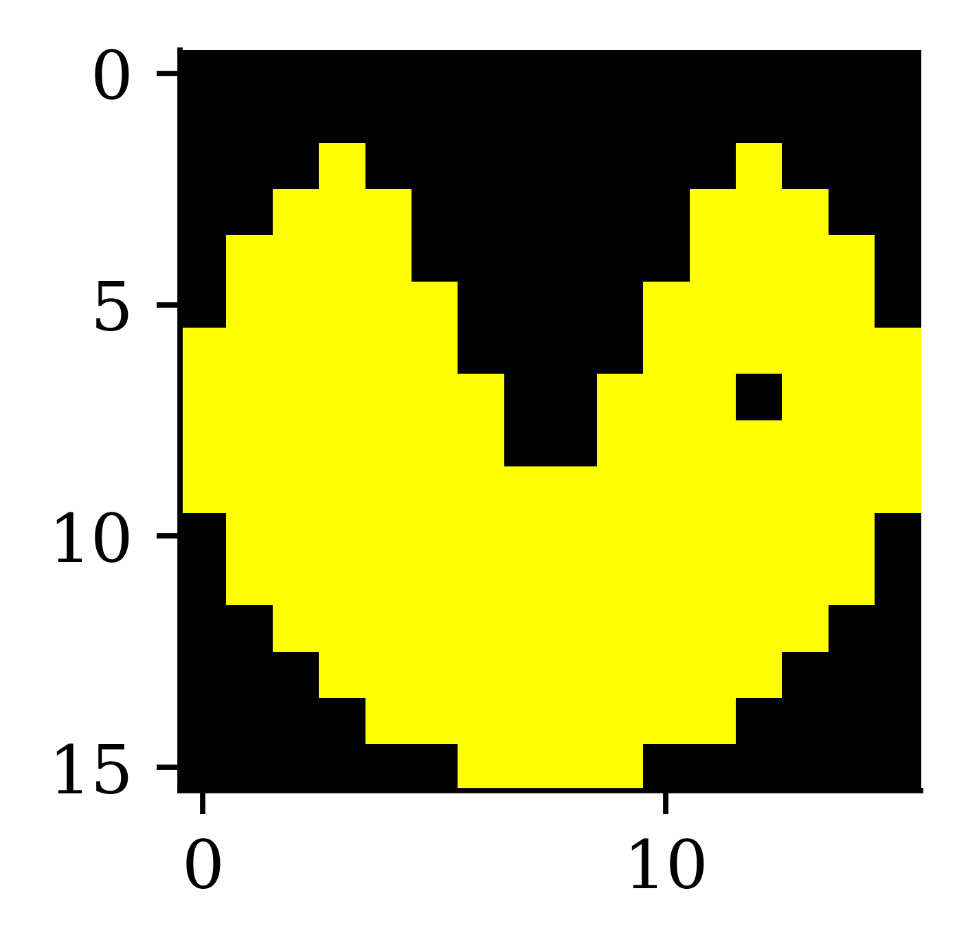

imshow(img3);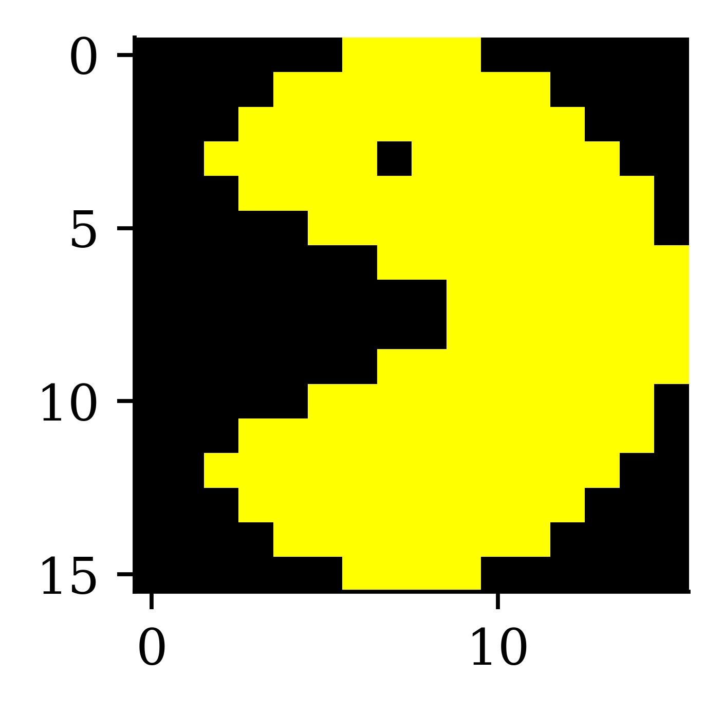

imshow(img4);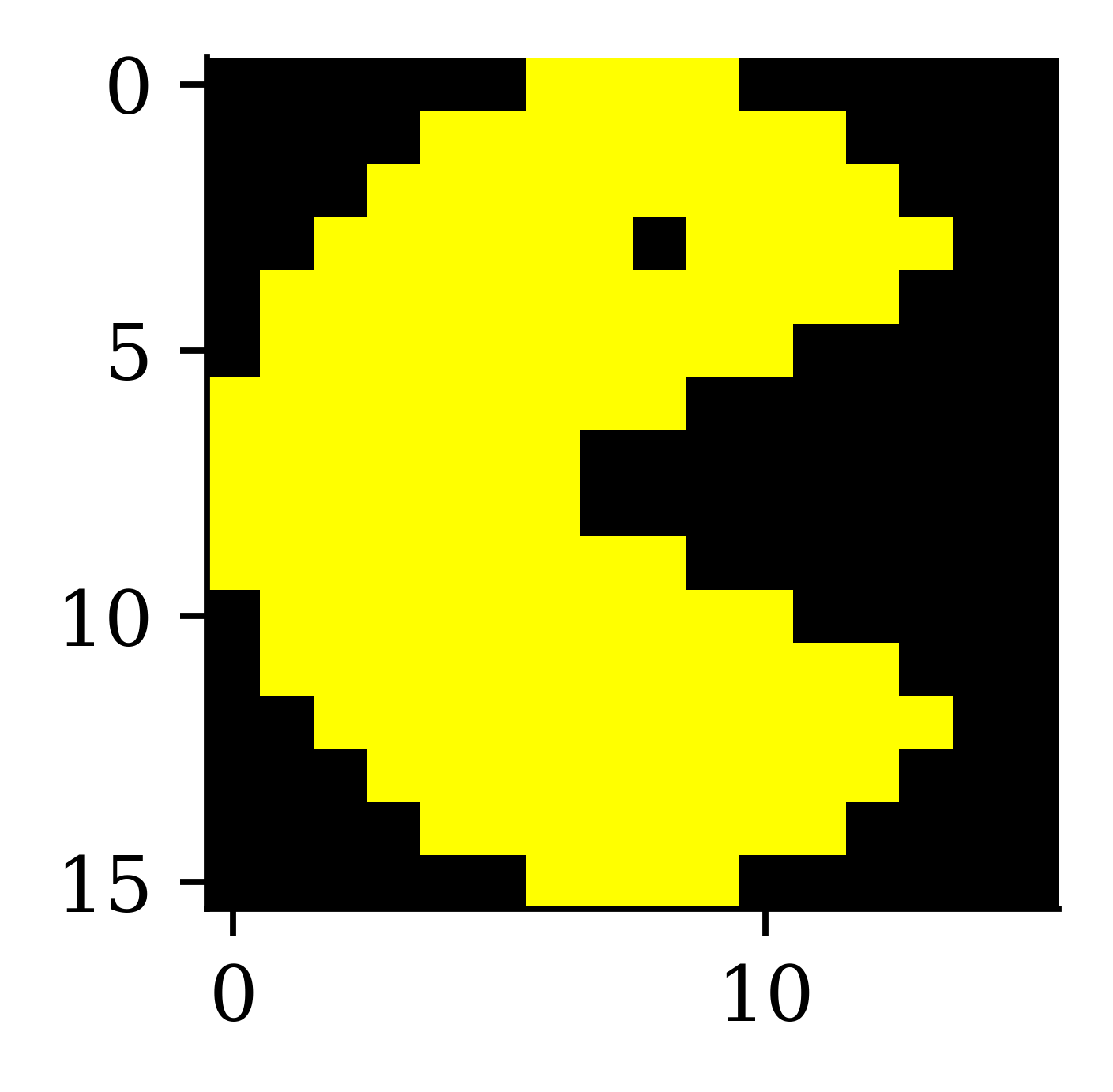

Why is 255 special?

Each pixel’s colour intensity is stored in one byte.

One byte is 8 bits, so in binary that is 00000000 to 11111111.

The largest unsigned number this can be is 2^8-1 = 255.

np.array([0, 1, 255, 256]).astype(np.uint8)

array([  0,   1, 255,   0], dtype=uint8)

If you had signed numbers, this would go from -128 to 127.

np.array([-128, 1, 127, 128]).astype(np.int8)

array([-128,    1,  127, -128], dtype=int8)

Alternatively, hexadecimal numbers are used. E.g. 10100001 is split into 1010 0001, and 1010=A, 0001=1, so combined it is 0xA1.

The Convolution Operation

The convolution operation

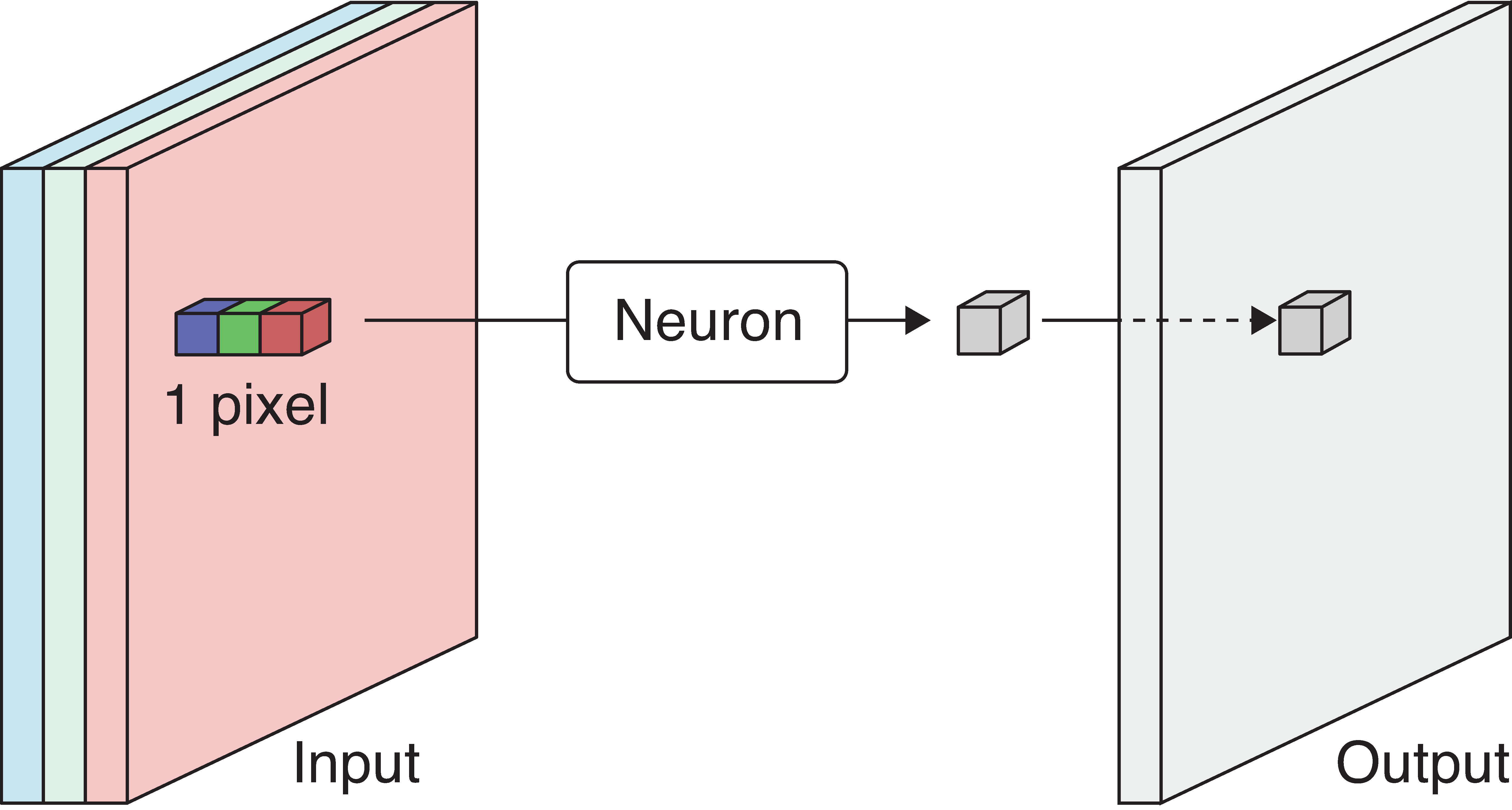
Scan the 3-channel input (colour image) with the neuron to produce a 1-channel output (grayscale image).

The output is produced by sweeping the neuron over the input. This is called convolution.

Aside: you’d have seen the convolution operation when calculating the density of S = X_1 + X_2 for i.i.d. X_1, X_2 \sim f_X as f_S(s) = \int f_X(x_1)\, f_X(s - x_1)\,\mathrm{d}x_1 = (f_X \star f_X)(s). This is why they’re named “convolutional”.

The weights and biases

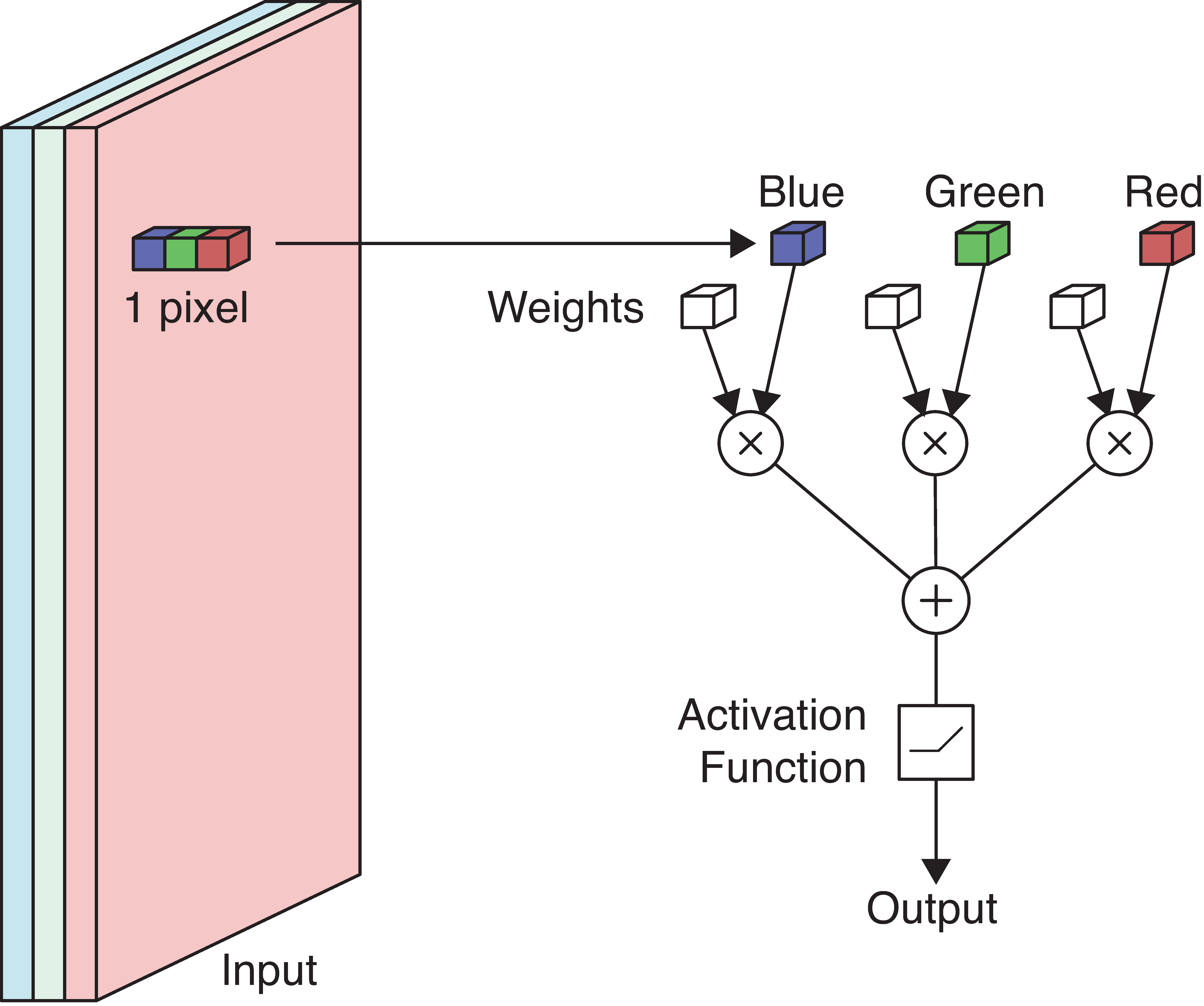
Example: Detecting yellow

Suppose we wish to detect if a picture has yellow colour in it. One option would be to apply a neuron over each pixel and see if it detects the colour yellow. We know that each pixel is represented by 3 numerical values that correspond to red, green and blue. Higher numeric values for red and green indicate higher chances of detecting yellow. Higher values for blue indicate lower chances of detecting yellow. Utilising this information, we can assign RGB weights to be 1, 1, -1 respectively.

Next, a standard multiplication between numeric values and weights is carried out, and the weighted sum is passed through the neuron.

If red/green \nearrow or blue \searrow then yellowness \nearrow. Set RGB weights to 1, 1, -1.

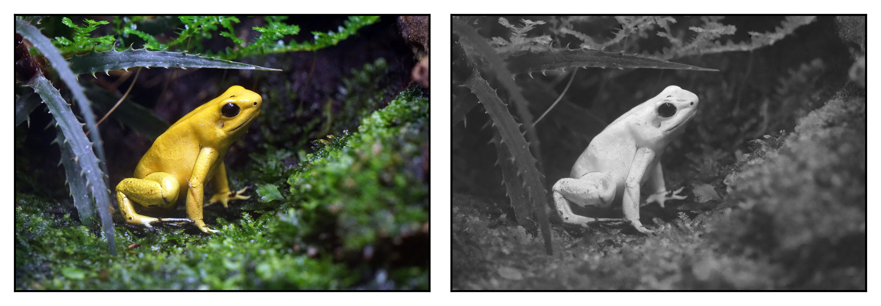
The following picture demonstrates how yellow-coloured areas (in the colour picture) are transformed into a white colour (in the greyscale picture). This is a result of the way we assigned the weights. Since we assigned +1 weights to red and green, and -1 to blue, it ended up resulting in large positive values (for the weighted sum) for the pixels in the yellow-coloured areas. Large positive values in the greyscale correspond to white colour. Therefore, the areas which were yellow in the colour picture converted to white in the greyscale. In practice, we do not manually assign weights, instead, we let the neural network decide the optimal weights during training.

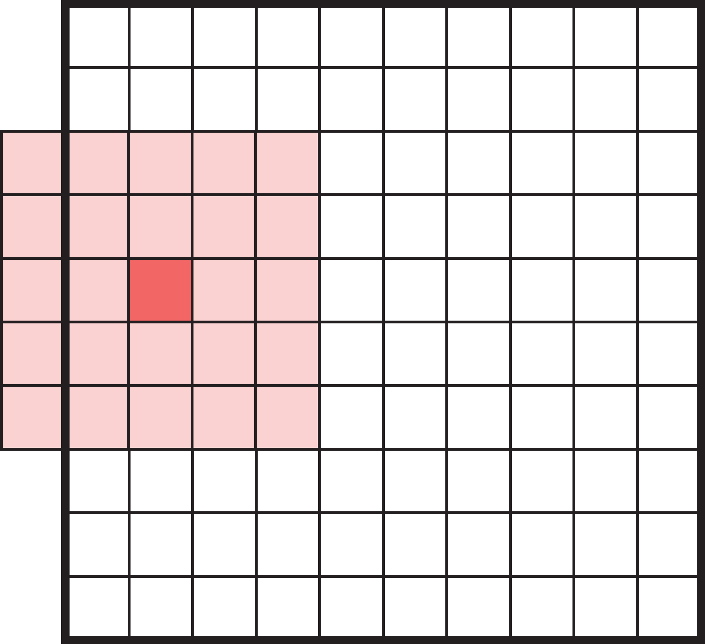
The more yellow the pixel in the colour image (left), the more white it is in the grayscale image.

This is about all we can detect by looking pixel-by-pixel. Typically we look at 3x3 or 5x5 blocks of pixels together.

Filters

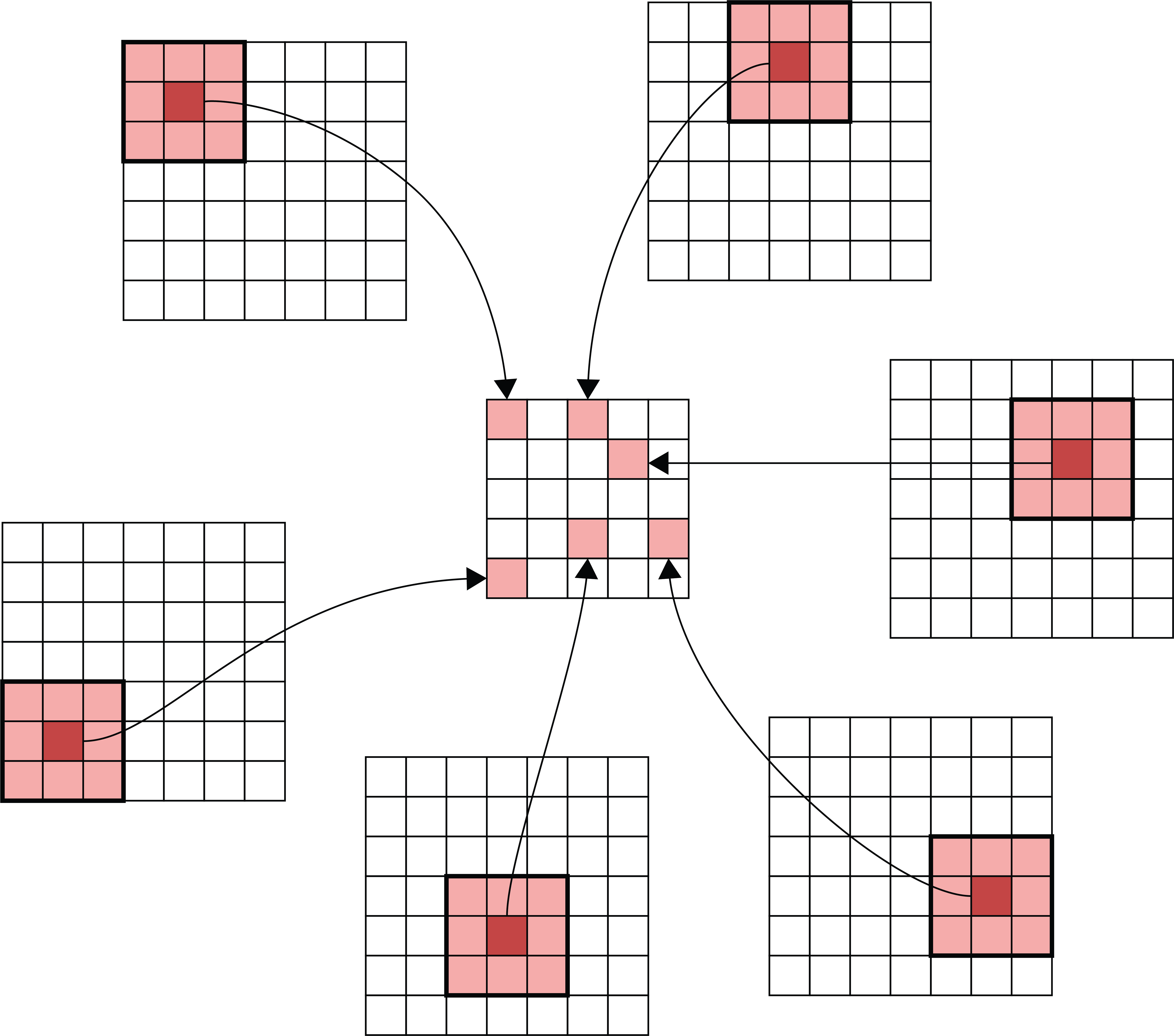
A *filter* (also called a *kernel*) is a small block of weights (plus a bias) which we sweep over the input in the convolution operation.

The patch of input pixels a filter covers at one location is its footprint. Applied there, the filter turns that patch into a single output number — which is exactly what one neuron does.
The same filter slides over every location instead of learning new weights per pixel. This weight sharing is why a convolution layer has so few parameters.

The above figure shows how 9 inputs transform into one output. As a result, dimensions of the output matrix is smaller than the dimensions of the input matrix. There are some options we can use if we wish to keep the size of input and output matrices same.

Example filter

An example of filter convolution in action.

Take a look at https://setosa.io/ev/image-kernels/.

Padding

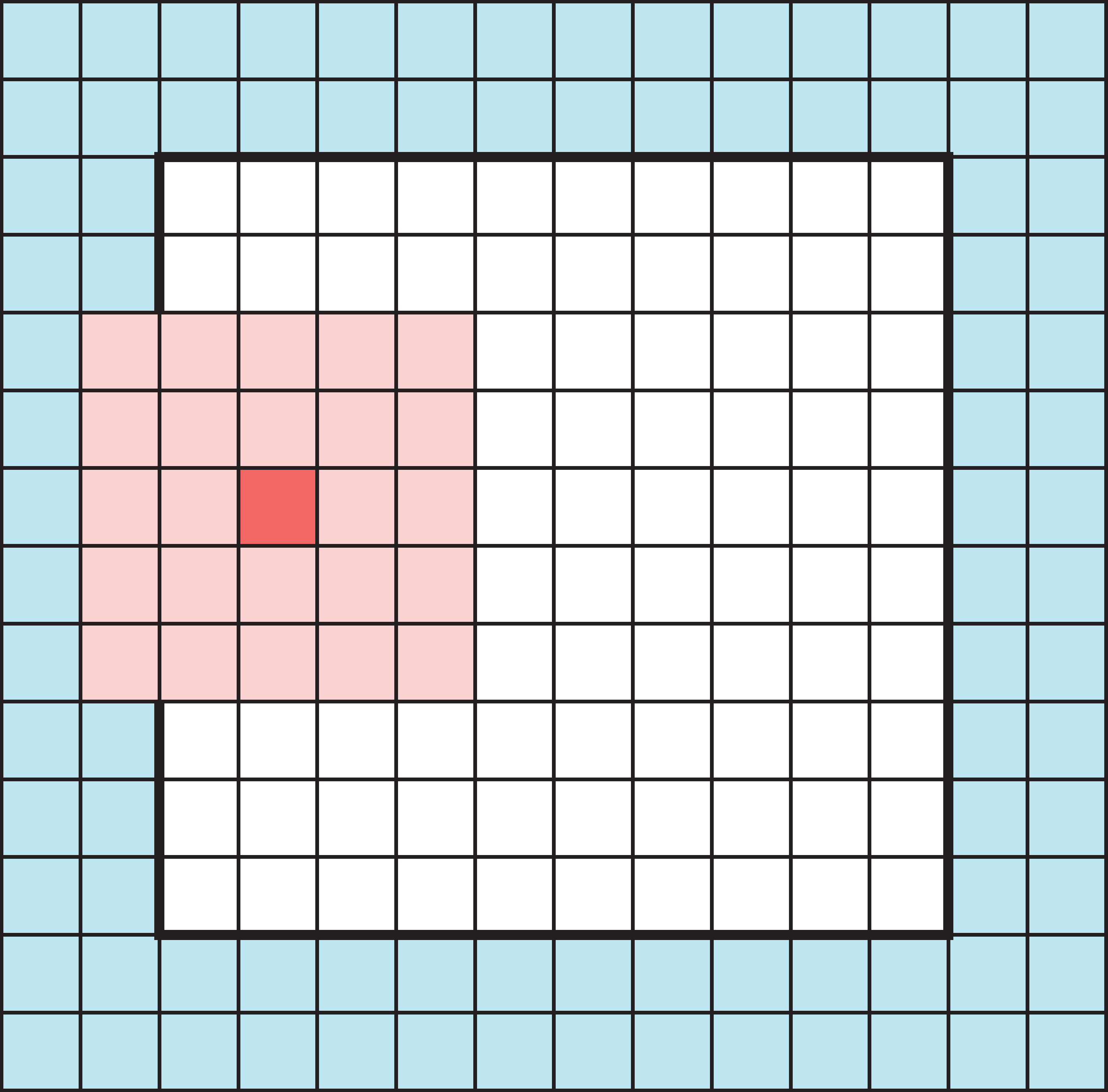
What happens when filters go off the edge of the input?

Add zeros around the input so the filter’s footprint doesn’t fall off the edge. This lets the output keep the same size as the input (padding="same").

Striding

Striding modifies how the filter moves across the image. Instead of moving one pixel at a time, we can take larger steps.

We don’t have to move the filter one pixel across/down at a time — a larger stride shrinks the output and saves computation.

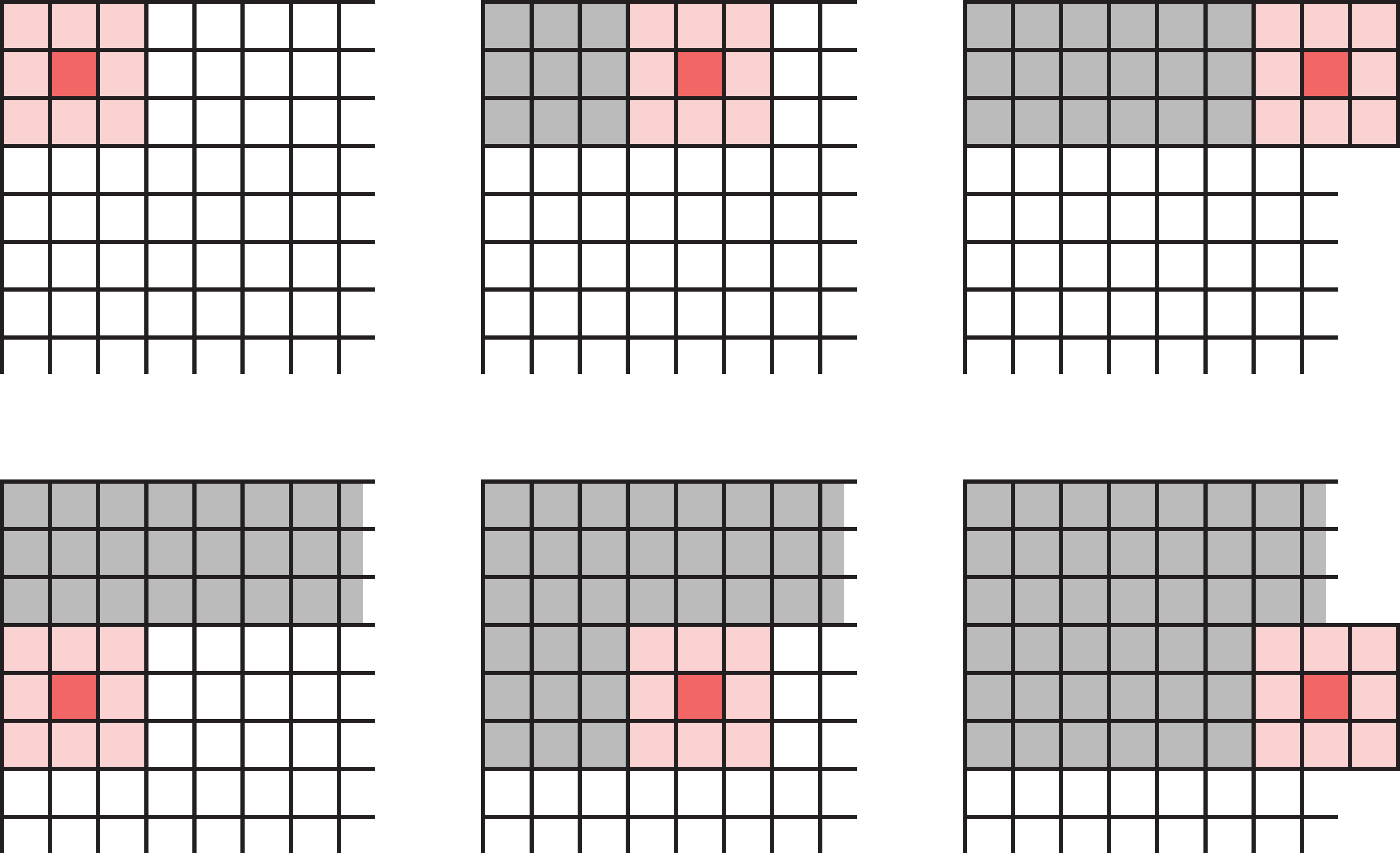
A 3x3 filter with stride 3 in both directions, so no input element is used more than once.

Multidimensional convolution

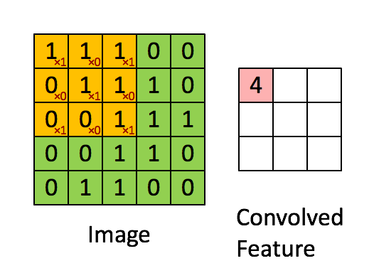
A filter covers a block of pixels (e.g. a 3x3 filter has 9 weights), and must have the same number of channels as its input.

A 3x3 filter over 3 channels: 27 weights.

In a multidimensional filter, the number of channels of the input must be equal to the number of channels in the filter (depths must be the same). The single-channel 3x3 filter has 9 weights; matching it to a 3-channel input gives 3x3x3 = 27 weights.

Example: 3x3 filter over RGB input

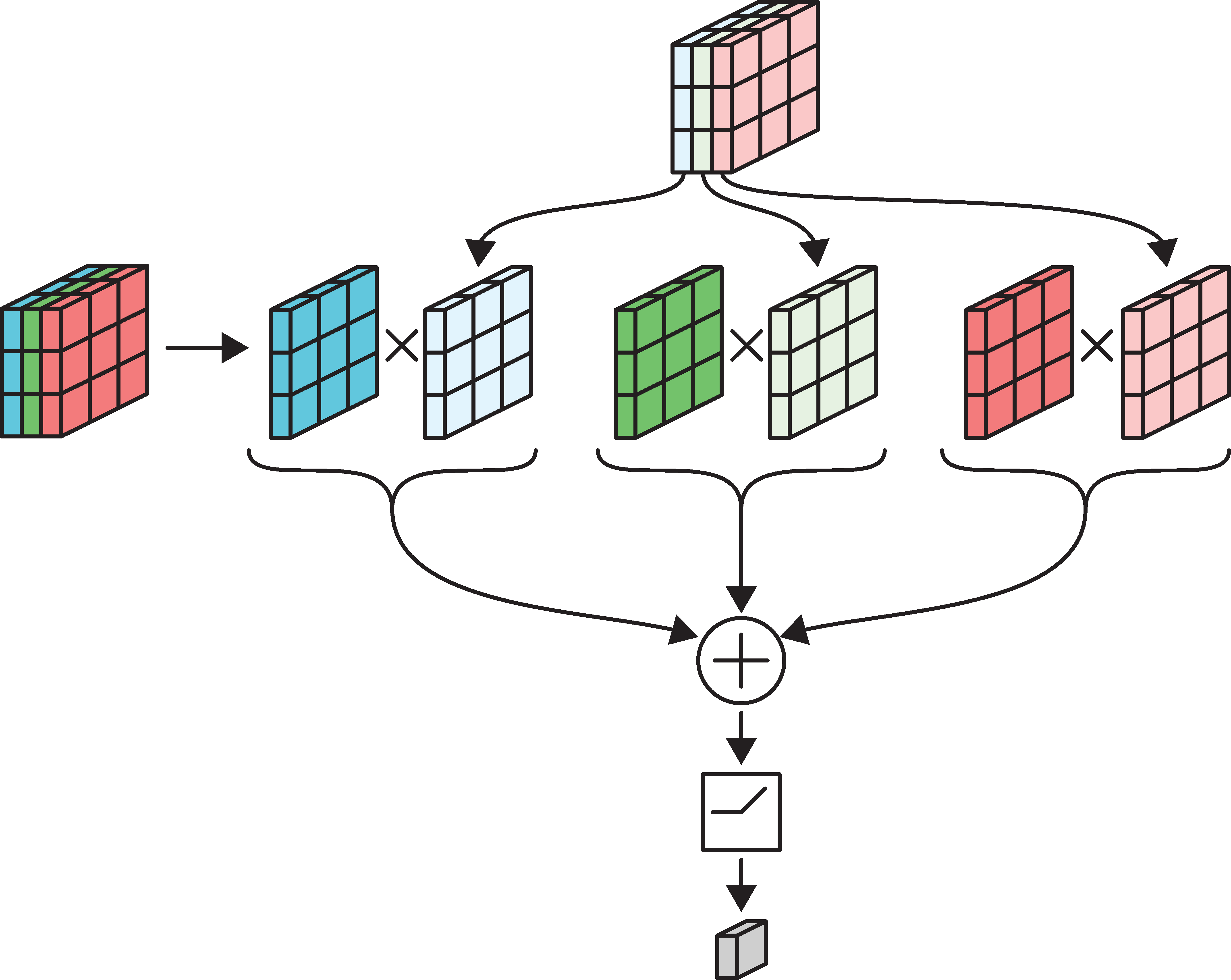
Each channel is multiplied separately & then added together.

The above figure shows how we pick a 3x3x3 block from the image, and then apply the 3x3 filter. The multiplication is carried out channel-wise, i.e. we select the first channel of the filter and the first channel of the image and carry out the element-wise multiplication. Once the elementwise multiplications for the three pairs of channels are completed, we sum them all, and pass through the neuron.

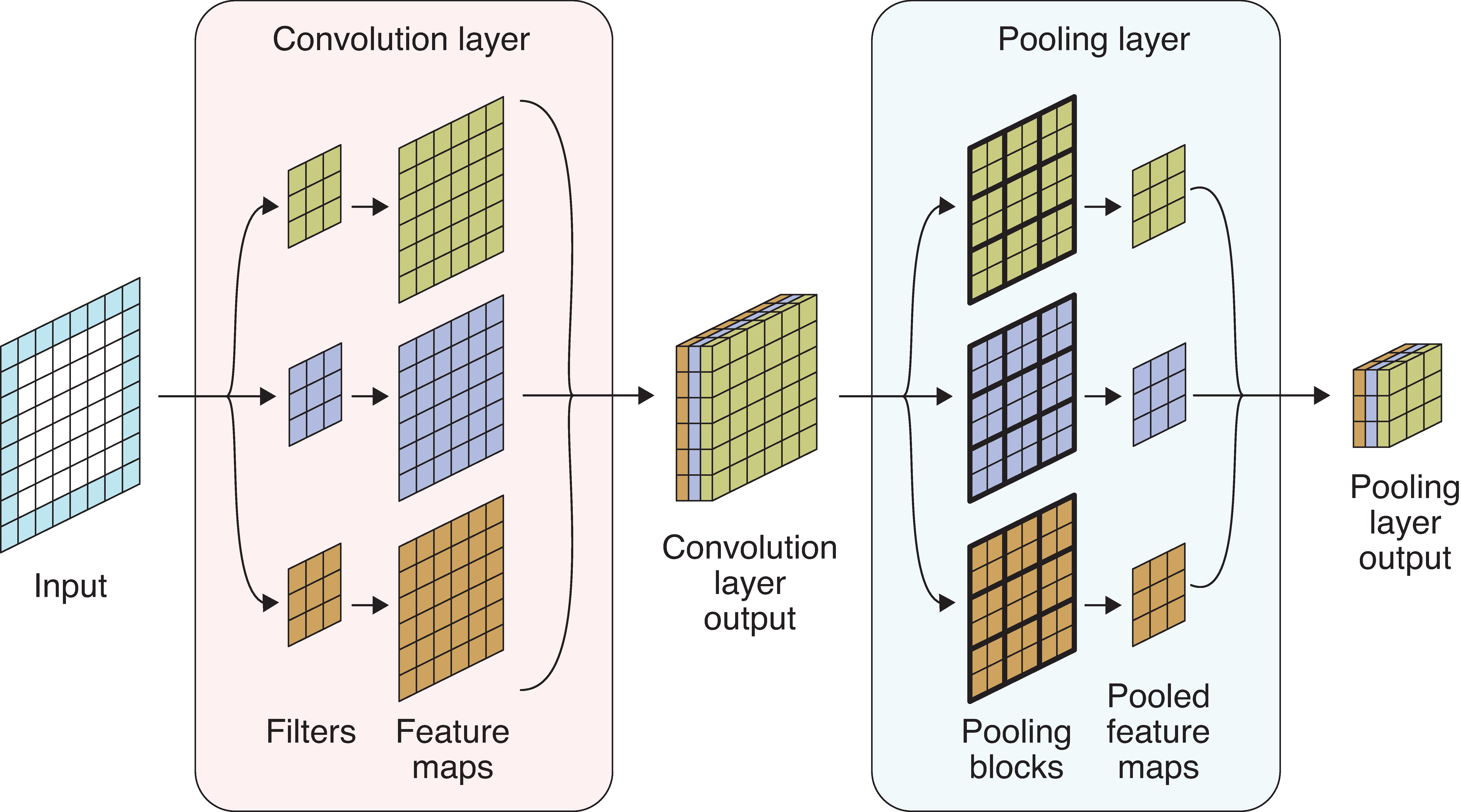
Convolution layer

Multiple filters are bundled together in one layer.
The filters are applied simultaneously and independently to the input.
Number of channels in the output will be the same as the number of filters.

The motivation behind applying filters simultaneously and independently is to let the filters learn different patterns in the input-output relationship. The idea is quite similar to using many neurons in one Dense layer (in a Dense layer, we would use multiple neurons so that different neurons can capture different patterns in the input-output relationship).

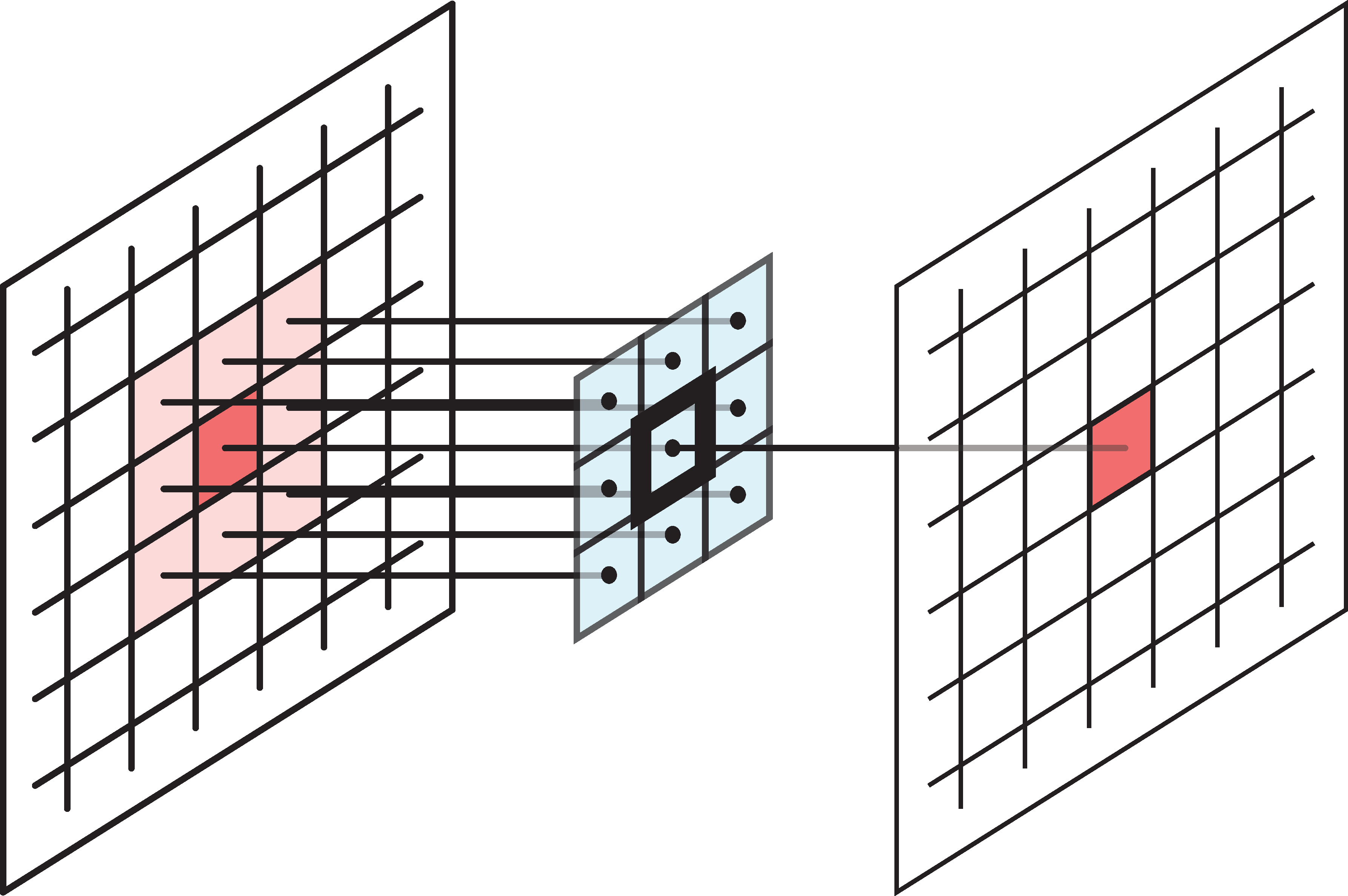
In the image:

6-channel input tensor
input pixels
four 3x3 filters
four output tensors
final output tensor.

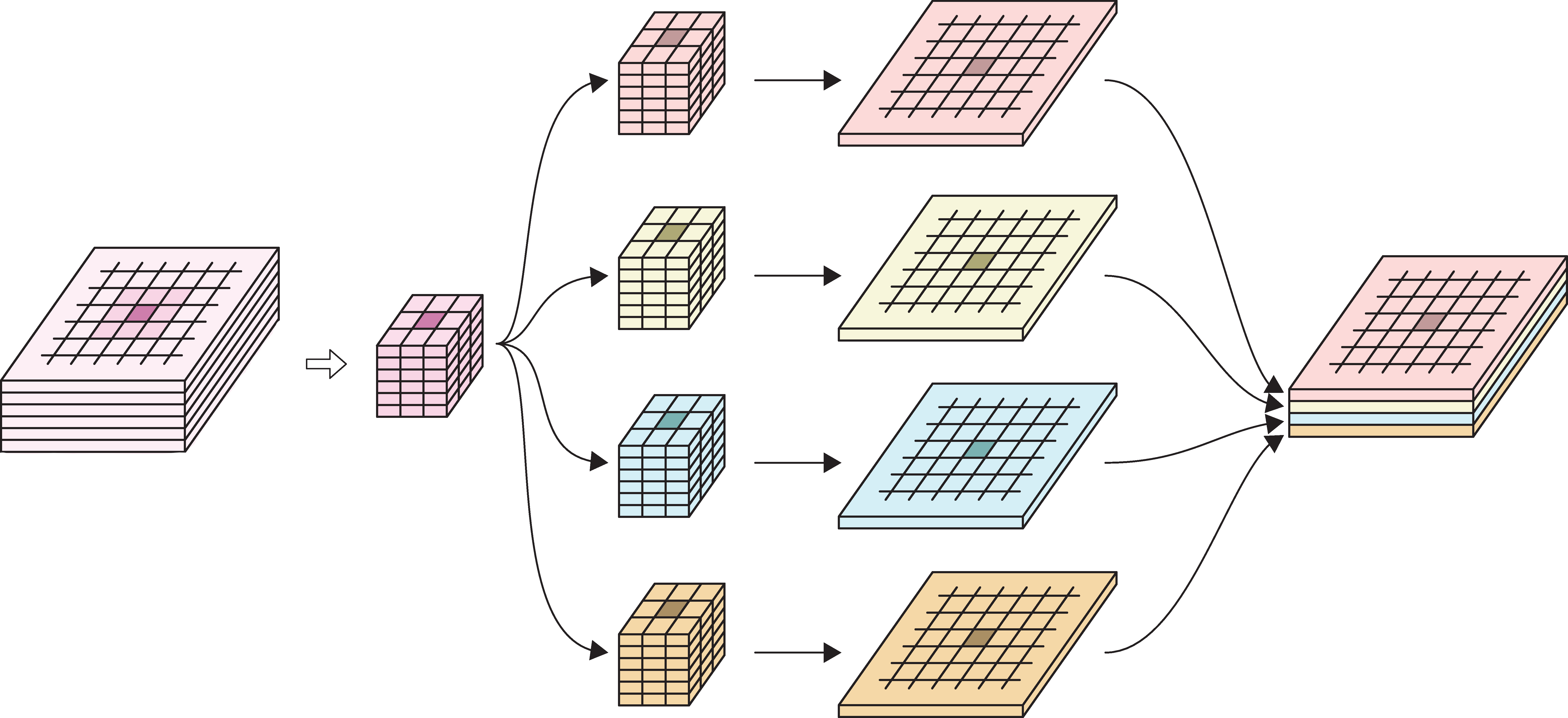
The above picture shows how we take in an image with 6 channels, select a 3x3 block (in pink colour), apply 4 different filters of same dimensions (in pink, green, blue and yellow), retrieve the output with 1 channel (1 output for each filter) and finally stack them together to create 1 output tensor. Note that the number of channels in the output tensor is 4, which is equal to the number of filters used.

Specifying a convolutional layer

Need to choose:

number of filters,
their size/footprint (e.g. 3x3, 5x5, etc.),
activation functions,
padding & striding (optional).

All the filter weights are learned during training.

Convolutional Neural Networks

A neural network that uses convolution layers is called a convolutional neural network.

A standard CNN architecture has the following components:

Input layer
Sequence of feature extraction layers (which combine convolution and pooling operations sequentially)
Sequence of classification layers (which include flattening and fully connected layers)
Final output layer

Convolution layers are used to extract meaningful patterns from the input using filters. Pooling layers are used to reduce the spatial dimensions of the feature maps generated from convolutional layers. The purpose of the feature extraction layers is to learn complex but meaningful, high levels patterns in data. The aim of classification layers is to receive the learned patterns and make decisions more closely related to the classification task at hand.

On a high level, as we move deeper into the network the number of channels (the depth) tends to grow while the spatial dimensions (height and width) of the feature maps shrink.

Pooling

Pooling, or downsampling, is a technique to blur a tensor.

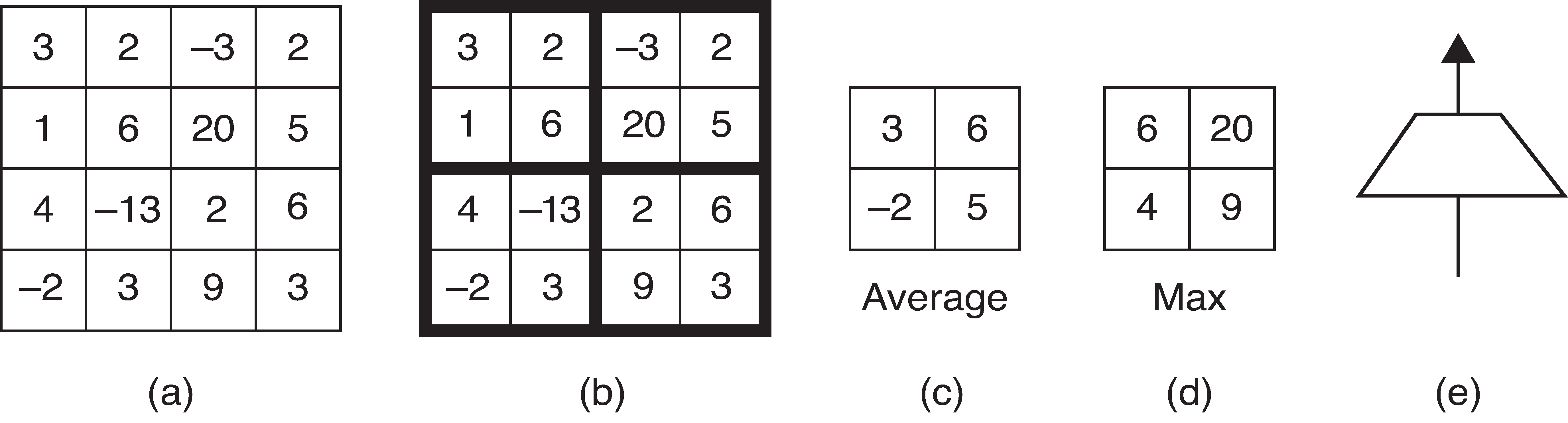
(a): Input tensor (b): Subdivide input tensor into 2x2 blocks (c): Average pooling (d): Max pooling (e): Icon for a pooling layer

Pooling for multiple channels

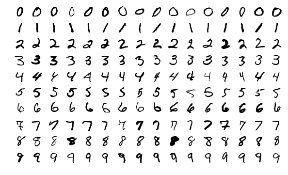
MNIST Dataset

LeNet-5 (1998)

Layer	Type	Channels	Size	Kernel size	Stride	Activation
In	Input	1	32×32	–	–	–
C1	Convolution	6	28×28	5×5	1	tanh
S2	Avg pooling	6	14×14	2×2	2	tanh
C3	Convolution	16	10×10	5×5	1	tanh
S4	Avg pooling	16	5×5	2×2	2	tanh
C5	Convolution	120	1×1	5×5	1	tanh
F6	Fully connected	–	84	–	–	tanh
Out	Fully connected	–	10	–	–	RBF

Note

MNIST images are 28×28 pixels, and with zero-padding (for a 5×5 kernel) that becomes 32×32.

AlexNet (2012)

Layer	Type	Channels	Size	Kernel	Stride	Padding	Activation
In	Input	3	227×227	–	–	–	–
C1	Convolution	96	55×55	11×11	4	valid	ReLU
S2	Max pool	96	27×27	3×3	2	valid	–
C3	Convolution	256	27×27	5×5	1	same	ReLU
S4	Max pool	256	13×13	3×3	2	valid	–
C5	Convolution	384	13×13	3×3	1	same	ReLU
C6	Convolution	384	13×13	3×3	1	same	ReLU
C7	Convolution	256	13×13	3×3	1	same	ReLU
S8	Max pool	256	6×6	3×3	2	valid	–
F9	Fully conn.	–	4,096	–	–	–	ReLU
F10	Fully conn.	–	4,096	–	–	–	ReLU
Out	Fully conn.	–	1,000	–	–	–	Softmax

Depth can be important for image tasks

Deeper models aren’t just better because they have more parameters.

Residual connection

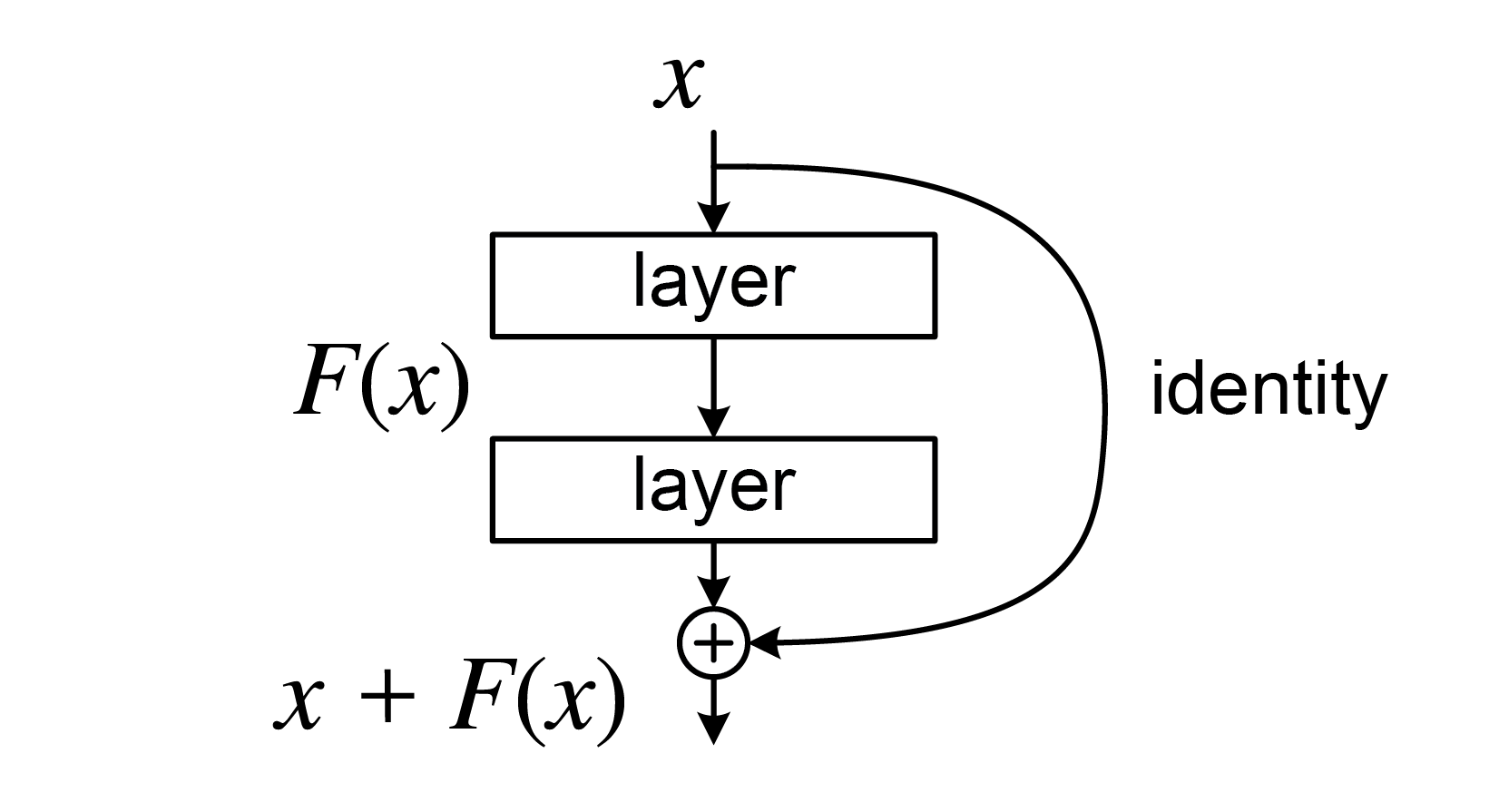
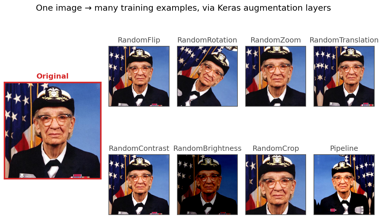
Image augmentation

Image augmentation: start with an image and create new training examples from it by applying small, label-preserving transformations. Examples include:

Flipping/rotating
Zooming/translating/cropping
Adjusting contrast/brightness

Image augmentation doesn’t add new information, but by training on many perturbed versions of each image it makes the model less sensitive to such small changes. In effect, the model has more images to learn from.

One image becomes many training examples, using Keras’ built-in augmentation layers.

What do the CNN layers learn?

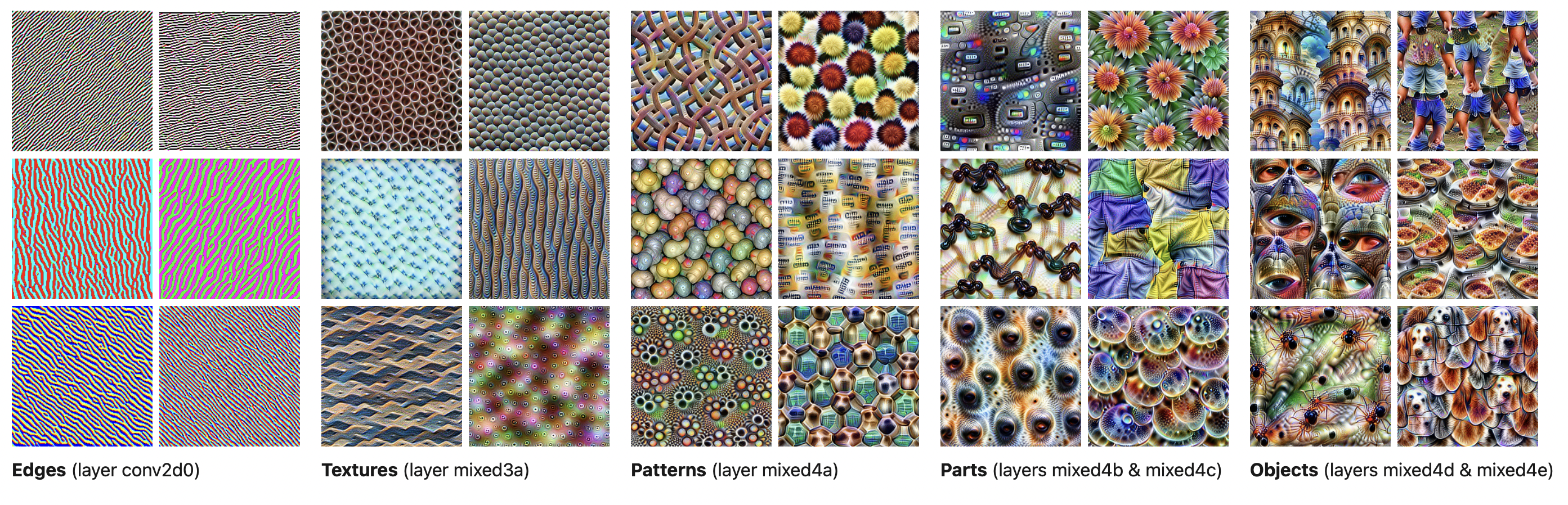
Early layers learn simple patterns; deep layers, complex ones.

CNN layers learn (sequentially):

Edges
Textures
Patterns
Parts
Objects

How does that work?

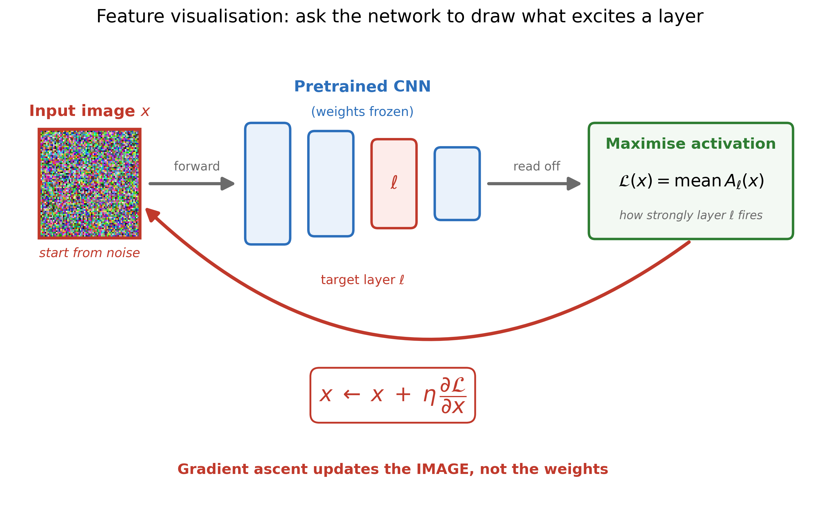
Start from a noise image and nudge its *pixels* until a chosen layer fires hardest.

The pictures above aren’t real photos — they’re synthesised by the network itself:

Take a pretrained CNN and freeze its weights.
Pick a target layer \ell, and start from a random-noise image x.
Run a forward pass and measure how strongly that layer fires, \mathcal{L}(x) = \mathrm{mean}\,A_\ell(x).
Backpropagate, but apply the update to the image rather than the weights: x \leftarrow x + \eta\,\tfrac{\partial \mathcal{L}}{\partial x} (gradient ascent, so the activation grows).
Repeat. The noise gradually morphs into the pattern that layer is most excited by.

The takeaway: early layers light up for simple things (edges, colours, textures), while deeper layers respond to complex things (parts, whole objects). (The real method also needs regularisation — jittering and rescaling the image each step — or it produces high-frequency junk instead of recognisable patterns.)

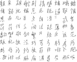
Chinese Character Recognition Dataset

CASIA Chinese handwriting database

Dataset source: Institute of Automation of Chinese Academy of Sciences (CASIA)

A 13 GB dataset of 3,999,571 handwritten characters.

Inspect a subset of characters

Pulling out 55 characters to experiment with.

人从众大夫天口太因鱼犬吠哭火炎啖木林森本竹羊美羔山出女囡鸟日东月朋明肉肤工白虎门闪问闲水牛马吗妈玉王国主川舟虫

Inspect directory structure

DisplayTree("CASIA-Dataset")

CASIA-Dataset/
├── Test/
│   ├── 东/
│   │   ├── 1.png
│   │   ├── 10.png
│   │   ├── 100.png
│   │   ├── 101.png
│   │   ├── 102.png
│   │   ├── 103.png
│   │   ├── 104.png
│   │   ├── 105.png
│   │   ├── 106.png
...
        ├── 97.png
        ├── 98.png
        └── 99.png

Count number of images for each character

def count_images_in_folders(root_folder):
    counts = {}
    for folder in root_folder.glob("*/"):
        counts[folder.name] = len(list(folder.glob("*.png")))
    return counts

train_counts = count_images_in_folders(Path("CASIA-Dataset/Train"))
test_counts = count_images_in_folders(Path("CASIA-Dataset/Test"))

print(train_counts)
print(test_counts)

{'哭': 584, '闪': 597, '马': 597, '啖': 240, '囡': 240, '明': 596, '太': 596, '森': 598, '国': 600, '女': 597, '本': 604, '夫': 599, '因': 603, '林': 598, '月': 604, '川': 593, '牛': 599, '鱼': 602, '玉': 602, '工': 600, '水': 597, '犬': 598, '肤': 601, '从': 598, '美': 591, '羔': 597, '鸟': 598, '肉': 598, '东': 601, '人': 597, '问': 601, '闲': 598, '日': 597, '竹': 600, '吠': 601, '门': 597, '吗': 596, '木': 598, '虎': 597, '大': 603, '天': 598, '妈': 595, '虫': 602, '白': 604, '朋': 595, '口': 597, '舟': 601, '山': 598, '王': 601, '众': 600, '羊': 600, '炎': 602, '出': 602, '主': 599, '火': 599}
{'哭': 138, '闪': 143, '马': 144, '啖': 60, '囡': 59, '明': 144, '太': 143, '森': 144, '国': 142, '女': 144, '本': 143, '夫': 141, '因': 144, '林': 143, '月': 144, '川': 142, '牛': 144, '鱼': 143, '玉': 142, '工': 141, '水': 143, '犬': 141, '肤': 140, '从': 142, '美': 144, '羔': 141, '鸟': 143, '肉': 143, '东': 142, '人': 144, '问': 143, '闲': 142, '日': 143, '竹': 142, '吠': 141, '门': 144, '吗': 143, '木': 144, '虎': 143, '大': 144, '天': 143, '妈': 142, '虫': 144, '白': 141, '朋': 144, '口': 143, '舟': 143, '山': 144, '王': 145, '众': 143, '羊': 144, '炎': 143, '出': 142, '主': 141, '火': 142}

Number of images for each character

plt.hist(train_counts.values(), bins=30, label="Train")
plt.hist(test_counts.values(), bins=30, label="Test")
plt.legend();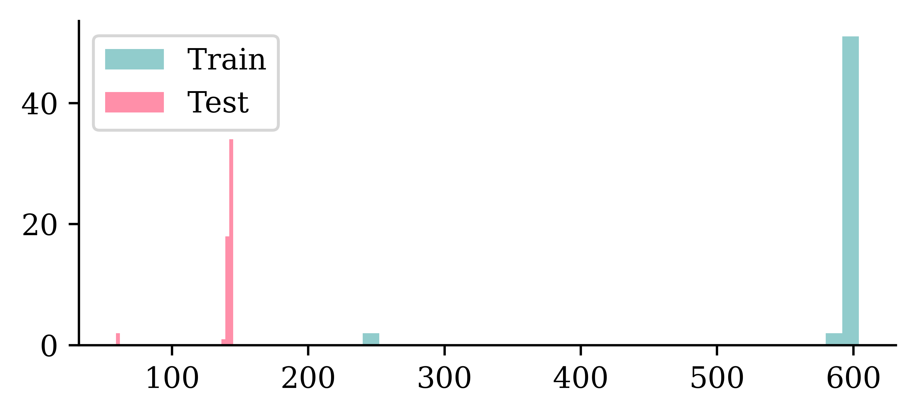

It differs, but basically ~600 training and ~140 test images per character. A couple of characters have a lot less of both though.

Checking the dimensions

Code

def get_image_dimensions(root_folder):
    dimensions = []
    for folder in root_folder.glob("*/"):
        for image in folder.glob("*.png"):
            img = imread(image)
            dimensions.append(img.shape)
    return dimensions

train_dimensions = get_image_dimensions(Path("CASIA-Dataset/Train"))
test_dimensions = get_image_dimensions(Path("CASIA-Dataset/Test"))

train_heights = [d[0] for d in train_dimensions]
train_widths = [d[1] for d in train_dimensions]
test_heights = [d[0] for d in test_dimensions]
test_widths = [d[1] for d in test_dimensions]

plt.hist(train_heights, bins=30, alpha=0.5, label="Train Heights")
plt.hist(train_widths, bins=30, alpha=0.5, label="Train Widths")
plt.hist(test_heights, bins=30, alpha=0.5, label="Test Heights")
plt.hist(test_widths, bins=30, alpha=0.5, label="Test Widths")
plt.legend();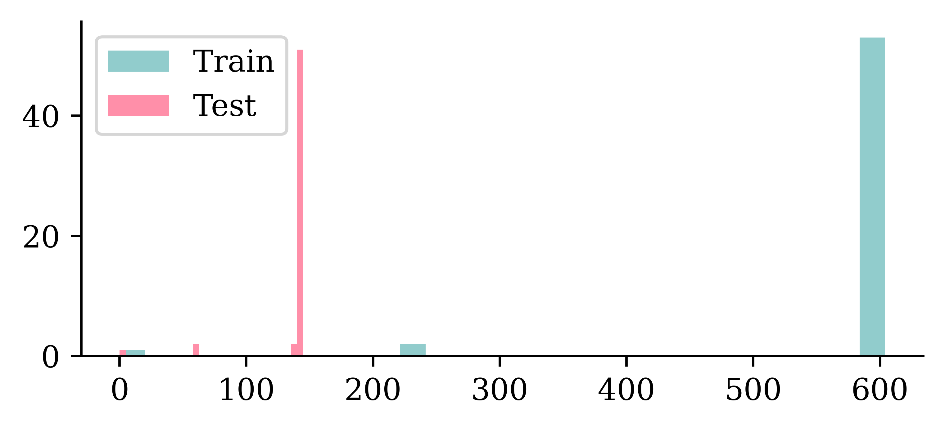

Checking the dimensions II

Using density=True removes the count imbalance, so we can compare the shapes of the distributions.

plt.hist(train_heights, bins=30, alpha=0.5, label="Train Heights", density=True)
plt.hist(test_heights, bins=30, alpha=0.5, label="Test Heights", density=True)
plt.legend();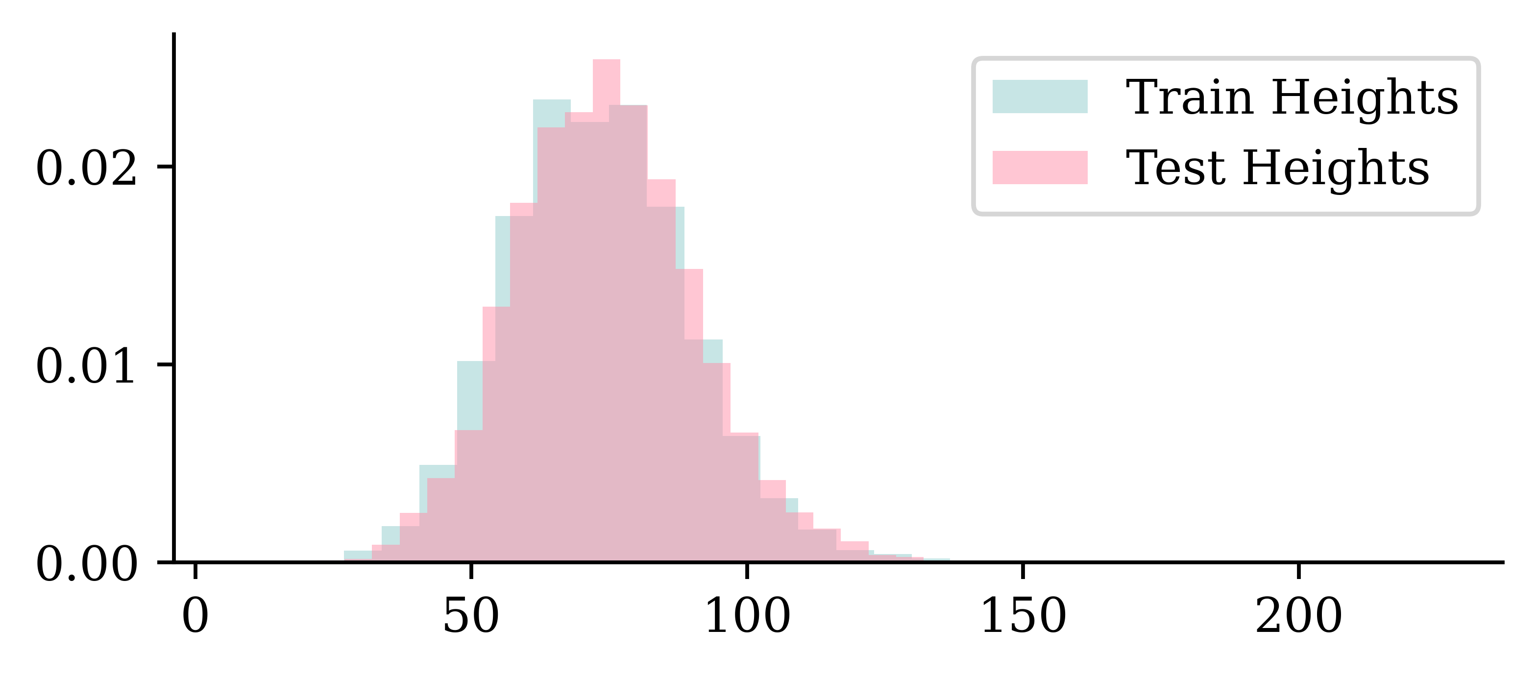

plt.hist(train_widths, bins=30, alpha=0.5, label="Train Widths", density=True)
plt.hist(test_widths, bins=30, alpha=0.5, label="Test Widths", density=True)
plt.legend();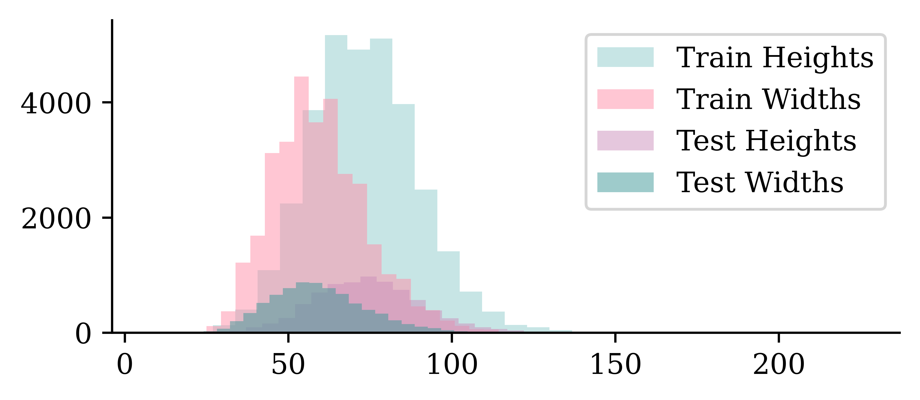

The images are taller than they are wide.
The distribution of dimensions are pretty similar between training and test sets.

Keras image dataset loading

Normally we’d used keras.utils.image_dataset_from_directory but the Chinese characters breaks it on Windows. I made an image loading function just for this demo.

Code

def preprocess_image(img_path, img_height=80, img_width=60):
    """
    Loads and preprocesses an image:
    - Converts to grayscale
    - Resizes to (img_height, img_width) using anti-aliasing
    - Returns a NumPy array normalized to [0,1]
    """
    img = Image.open(img_path).convert("L")  # Open image and convert to grayscale
    img = img.resize((img_width, img_height), Image.LANCZOS)  # Resize with anti-aliasing
    return np.array(img, dtype=np.float32)

def load_images_from_directory(directory, img_height=80, img_width=60):
    """
    Loads images and labels from a directory where each subfolder represents a class.
    
    Returns:
        X (numpy array): Image data of shape (num_samples, img_height, img_width, 1).
        y (numpy array): Labels as integer indices.
        class_names (list): List of class names in sorted order.
    """
    directory = Path(directory)  # Ensure it's a Path object
    class_names = sorted([d.name for d in directory.iterdir() if d.is_dir()])  # Sorted UTF-8 class names
    class_name_to_index = {name: i for i, name in enumerate(class_names)}

    image_paths, labels = [], []
    
    for class_name in class_names:
        class_dir = directory / class_name
        for img_path in sorted(class_dir.glob("*.png")):
            image_paths.append(img_path)
            labels.append(class_name_to_index[class_name])

    # Load and preprocess images
    X = np.array([preprocess_image(img, img_height, img_width) for img in image_paths])
    X = X[..., np.newaxis]  # Add channel dimension
    y = np.array(labels, dtype=np.int32)

    return X, y, class_names

data_dir = Path("CASIA-Dataset")
img_height, img_width = 80, 60  # Target image size

# Load 'training' and test datasets
X_main, y_main, class_names = load_images_from_directory(data_dir / "Train", img_height, img_width)
X_test, y_test, _ = load_images_from_directory(data_dir / "Test", img_height, img_width)

# Verify dataset shape
print(f"Train: X={X_main.shape}, y={y_main.shape}")
print(f"Test: X={X_test.shape}, y={y_test.shape}")
print("Class Names:", class_names)

Train: X=(32206, 80, 60, 1), y=(32206,)
Test: X=(7684, 80, 60, 1), y=(7684,)
Class Names: ['东', '主', '人', '从', '众', '出', '口', '吗', '吠', '哭', '啖', '因', '囡', '国', '大', '天', '太', '夫', '女', '妈', '山', '川', '工', '日', '明', '月', '朋', '木', '本', '林', '森', '水', '火', '炎', '牛', '犬', '玉', '王', '白', '竹', '羊', '美', '羔', '肉', '肤', '舟', '虎', '虫', '门', '闪', '问', '闲', '马', '鱼', '鸟']

The shape of the X data represents:

Number of images
Image height
Image width
Image depth

Some setup

Split the data into training and validation.

X_train, X_val, y_train, y_val = train_test_split(X_main, y_main, test_size=0.2,
    random_state=123)
print(X_train.shape, y_train.shape, X_val.shape, y_val.shape, X_test.shape, y_test.shape)

(25764, 80, 60, 1) (25764,) (6442, 80, 60, 1) (6442,) (7684, 80, 60, 1) (7684,)

CHINESE_FONT = fm.FontProperties(fname="STHeitiTC-Medium-01.ttf")

def plot_mandarin_characters(X, y, class_names, n=5, title_font=CHINESE_FONT):
    # Plot the first n images in X
    plt.figure(figsize=(10, 4))
    for i in range(n):
        plt.subplot(1, n, i + 1)
        plt.imshow(X[i], cmap="gray")
        plt.title(class_names[y[i]], fontproperties=title_font)
        plt.axis("off")

class_names[:5]

['东', '主', '人', '从', '众']

X_dong = X_train[y_train == 0]; y_dong = y_train[y_train == 0]
X_ren = X_train[y_train == 2]; y_ren = y_train[y_train == 2]

Plotting some training characters

Code

plot_mandarin_characters(X_dong, y_dong, class_names)

Code

plot_mandarin_characters(X_ren, y_ren, class_names)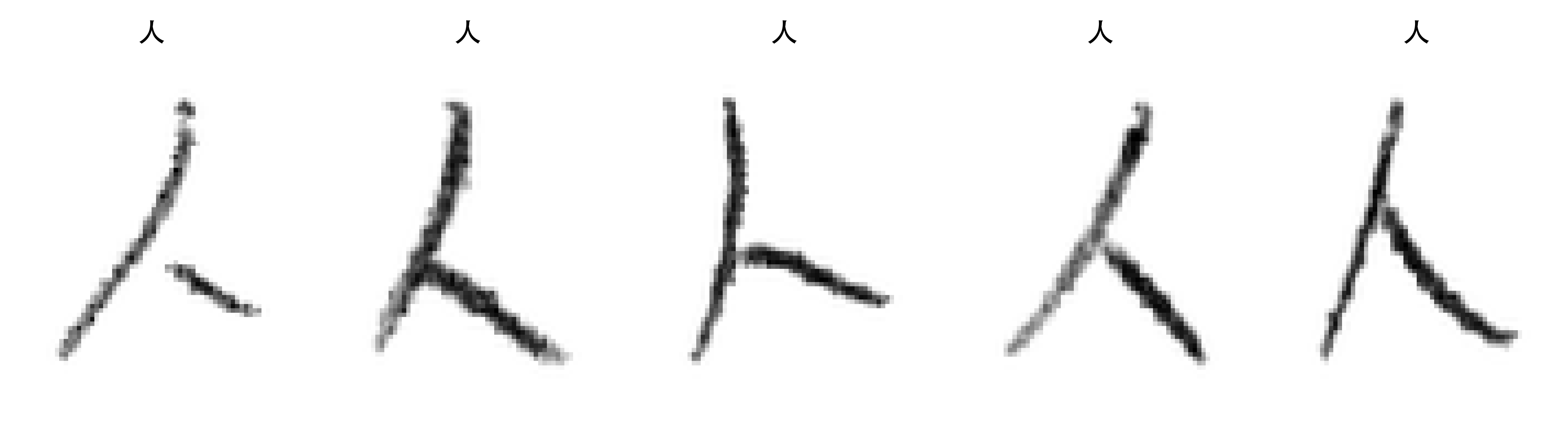

Without the colourmap..

dong = X_test[y_test == 0][0]
plt.imshow(dong, cmap="gray");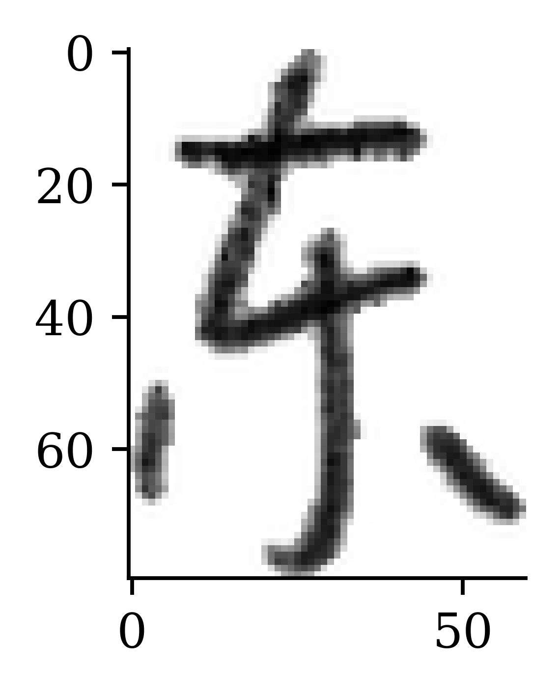

dong = X_test[y_test == 0][1]
plt.imshow(dong);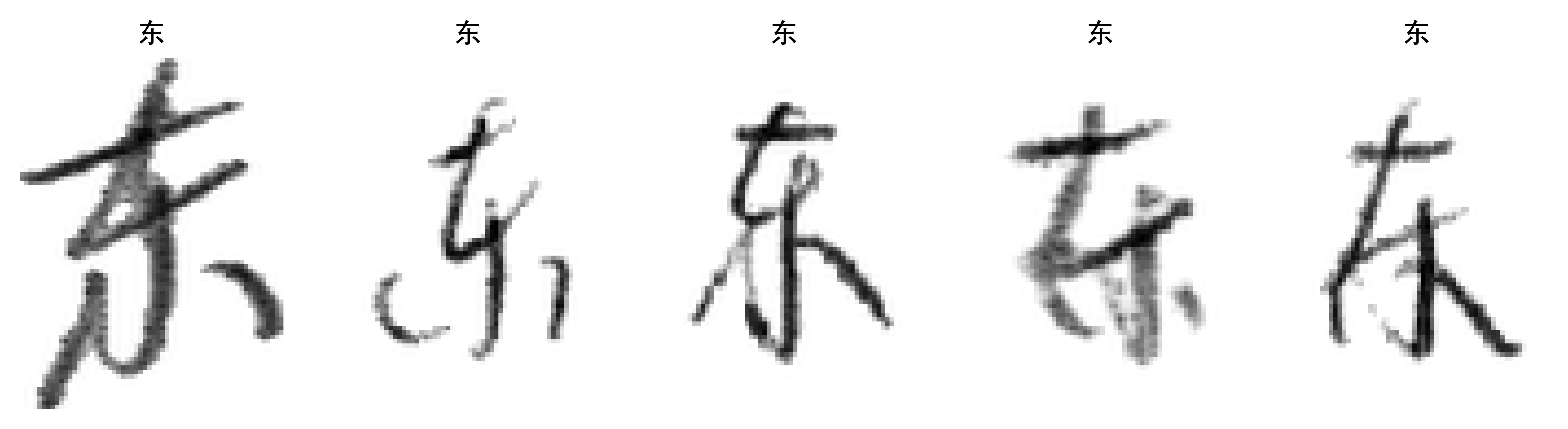

Training Our Models

Make simple baseline (multinomial) logistic regression

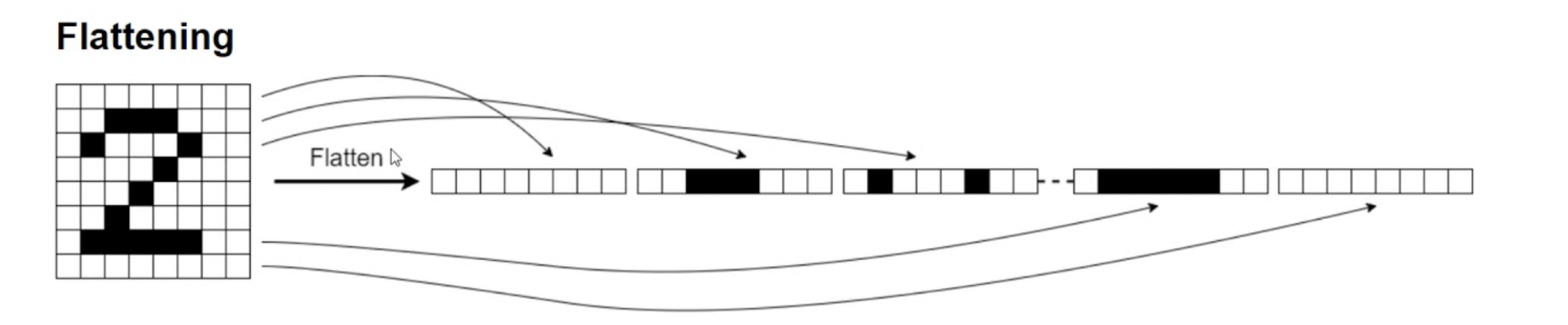
By flattening the image, we convert the 2D grid of pixels (a rank-2 tensor) into a single long vector (a rank-1 tensor), turning the dataset into a tabular one. The pixel values are all still there, but the model loses track of which pixels were neighbours — it can no longer exploit the 2D spatial structure that convolution relies on.

1num_classes = np.unique(y_train).shape[0]
random.seed(123)
model = Sequential([
  Input((img_height, img_width, 1)), Flatten(), Rescaling(1./255),
  Dense(num_classes, activation="softmax")
])

1: Specifies the number of unique categories in the train set

Tip

The Rescaling layer will rescale the intensities to [0, 1].

Inspecting the model

model.summary()

Model: "sequential"

┏━━━━━━━━━━━━━━━━━━━━━━━━━━━━━━━━━┳━━━━━━━━━━━━━━━━━━━━━━━━┳━━━━━━━━━━━━━━━┓
┃ Layer (type)                    ┃ Output Shape           ┃       Param # ┃
┡━━━━━━━━━━━━━━━━━━━━━━━━━━━━━━━━━╇━━━━━━━━━━━━━━━━━━━━━━━━╇━━━━━━━━━━━━━━━┩
│ flatten (Flatten)               │ (None, 4800)           │             0 │
├─────────────────────────────────┼────────────────────────┼───────────────┤
│ rescaling (Rescaling)           │ (None, 4800)           │             0 │
├─────────────────────────────────┼────────────────────────┼───────────────┤
│ dense (Dense)                   │ (None, 55)             │       264,055 │
└─────────────────────────────────┴────────────────────────┴───────────────┘

 Total params: 264,055 (1.01 MB)

 Trainable params: 264,055 (1.01 MB)

 Non-trainable params: 0 (0.00 B)

Plot the model

plot_model(model, show_shapes=True)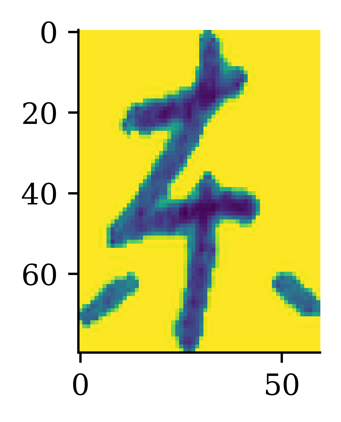

Fitting the model

loss = keras.losses.SparseCategoricalCrossentropy()
topk = keras.metrics.SparseTopKCategoricalAccuracy(k=5)
1model.compile(optimizer='adam', loss=loss, metrics=['accuracy', topk])

es = EarlyStopping(patience=15, restore_best_weights=True,
2    monitor="val_accuracy", verbose=2)
hist = model.fit(X_train, y_train, validation_data=(X_val, y_val),
3    epochs=100, batch_size=128, callbacks=[es], verbose=0)
history = hist.history

1: Compile the model with specified optimizer ("adam") and loss function (cross-entropy). The metrics we look at are accuracy and top-5 accuracy
2: Perform early stopping to fit the parameters, using the accuracy on the validation set to determine the stopping point
3: Fit the model with the optimized parameters

Plot the loss/accuracy curves

Code

def plot_history(history):
    epochs = range(len(history["loss"]))

    plt.subplot(1, 2, 1)
    plt.plot(epochs, history["accuracy"], label="Train")
    plt.plot(epochs, history["val_accuracy"], label="Val")
    plt.legend(loc="lower right")
    plt.title("Accuracy")

    plt.subplot(1, 2, 2)
    plt.plot(epochs, history["loss"], label="Train")
    plt.plot(epochs, history["val_loss"], label="Val")
    plt.legend(loc="upper right")
    plt.title("Loss")
    plt.show()

plot_history(history)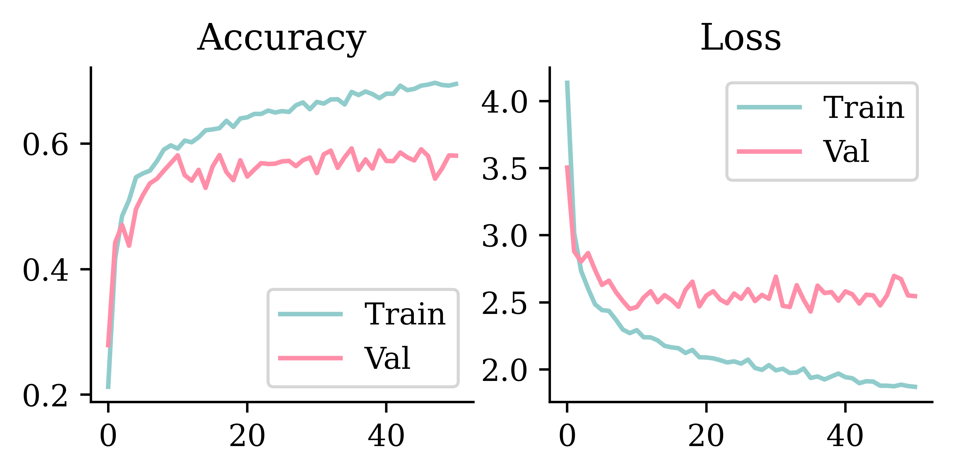

Look at the metrics

print(model.evaluate(X_train, y_train, verbose=0))
print(model.evaluate(X_val, y_val, verbose=0))

[1.8805104494094849, 0.6948843598365784, 0.8843735456466675]
[2.431033134460449, 0.592362642288208, 0.8346786499023438]

loss_value, accuracy, top5_accuracy = model.evaluate(X_val, y_val, verbose=0)
print(f"Validation Loss: {loss_value:.4f}")
print(f"Validation Accuracy: {accuracy:.4f}")
print(f"Validation Top 5 Accuracy: {top5_accuracy:.4f}")

Validation Loss: 2.4310
Validation Accuracy: 0.5924
Validation Top 5 Accuracy: 0.8347

Note

Why is top-5 accuracy greater than accuracy?

Accuracy: the proportion of guesses that are correct (the “guess” is the category with the highest implied probability)
Top-5 accuracy: the proportion of the time that the top 5 categories (the 5 categories with the highest implied probabilities) include the correct answer

Make a CNN

random.seed(123)

model = Sequential([
  Input((img_height, img_width, 1)),
1  Rescaling(1./255),
2  Conv2D(16, 3, padding="same", activation="relu", name="conv1"),
3  MaxPooling2D(name="pool1"),
  Conv2D(32, 3, padding="same", activation="relu", name="conv2"),
  MaxPooling2D(name="pool2"),
  Conv2D(64, 3, padding="same", activation="relu", name="conv3"),
  MaxPooling2D(name="pool3", pool_size=(4, 4)),
4  Flatten(),
  Dense(64, activation="relu"),
  Dense(num_classes)           
])

1: Rescales the numeric representations of data which ranges from [0,255] into [0, 1] range
2: Applies the convolution layer. Here padding="same" ensures that the dimensions of the input and output matrices remain same
3: Applies MaxPooling, which reduces the spatial dimensions by carrying forward the maximum value over an input window
4: Applies the Flatten layer to convert the 2D array (from pooling) into a single column vector, and passes through couple of Dense layers to train the neural network for the specific classification problem. Note that the output layer has number of neurons equal to num_classes, which corresponds to the number of unique classes in the output.

Inspect the model

model.summary()

Model: "sequential_1"

┏━━━━━━━━━━━━━━━━━━━━━━━━━━━━━━━━━┳━━━━━━━━━━━━━━━━━━━━━━━━┳━━━━━━━━━━━━━━━┓
┃ Layer (type)                    ┃ Output Shape           ┃       Param # ┃
┡━━━━━━━━━━━━━━━━━━━━━━━━━━━━━━━━━╇━━━━━━━━━━━━━━━━━━━━━━━━╇━━━━━━━━━━━━━━━┩
│ rescaling_1 (Rescaling)         │ (None, 80, 60, 1)      │             0 │
├─────────────────────────────────┼────────────────────────┼───────────────┤
│ conv1 (Conv2D)                  │ (None, 80, 60, 16)     │           160 │
├─────────────────────────────────┼────────────────────────┼───────────────┤
│ pool1 (MaxPooling2D)            │ (None, 40, 30, 16)     │             0 │
├─────────────────────────────────┼────────────────────────┼───────────────┤
│ conv2 (Conv2D)                  │ (None, 40, 30, 32)     │         4,640 │
├─────────────────────────────────┼────────────────────────┼───────────────┤
│ pool2 (MaxPooling2D)            │ (None, 20, 15, 32)     │             0 │
├─────────────────────────────────┼────────────────────────┼───────────────┤
│ conv3 (Conv2D)                  │ (None, 20, 15, 64)     │        18,496 │
├─────────────────────────────────┼────────────────────────┼───────────────┤
│ pool3 (MaxPooling2D)            │ (None, 5, 3, 64)       │             0 │
├─────────────────────────────────┼────────────────────────┼───────────────┤
│ flatten_1 (Flatten)             │ (None, 960)            │             0 │
├─────────────────────────────────┼────────────────────────┼───────────────┤
│ dense_1 (Dense)                 │ (None, 64)             │        61,504 │
├─────────────────────────────────┼────────────────────────┼───────────────┤
│ dense_2 (Dense)                 │ (None, 55)             │         3,575 │
└─────────────────────────────────┴────────────────────────┴───────────────┘

 Total params: 88,375 (345.21 KB)

 Trainable params: 88,375 (345.21 KB)

 Non-trainable params: 0 (0.00 B)

Plot the CNN

plot_model(model, show_shapes=True)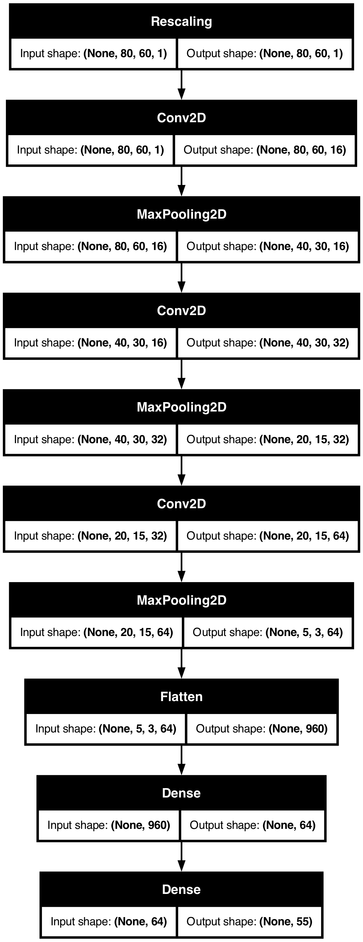

Source: Randall Munroe (2019), xkcd #2173: Trained a Neural Net.

Fit the CNN

1loss = keras.losses.SparseCategoricalCrossentropy(from_logits=True)
2topk = keras.metrics.SparseTopKCategoricalAccuracy(k=5)
3model.compile(optimizer='adam', loss=loss, metrics=['accuracy', topk])

es = EarlyStopping(patience=15, restore_best_weights=True,
    monitor="val_accuracy", verbose=2)
hist = model.fit(X_train, y_train, validation_data=(X_val, y_val),
    epochs=100, batch_size=128, callbacks=[es], verbose=0)
history = hist.history

1: Defines the loss function with an added command from_logits=True. Doing this instead of defining a softmax function at the output Dense layer of the neural network is expected to be more numerically stable
2: Specifies a new metric to keep track of accuracy of the top 5 predicted classes. This means that, for each input image, the metric will consider whether the true class is among the top 5 predicted classes by the model
3: Compiles the model as usual with an optimizer, a loss function and metrics to monitor

Tip

Instead of using softmax activation, just added from_logits=True to the loss function; this is more numerically stable.

Plot the loss/accuracy curves

plot_history(history)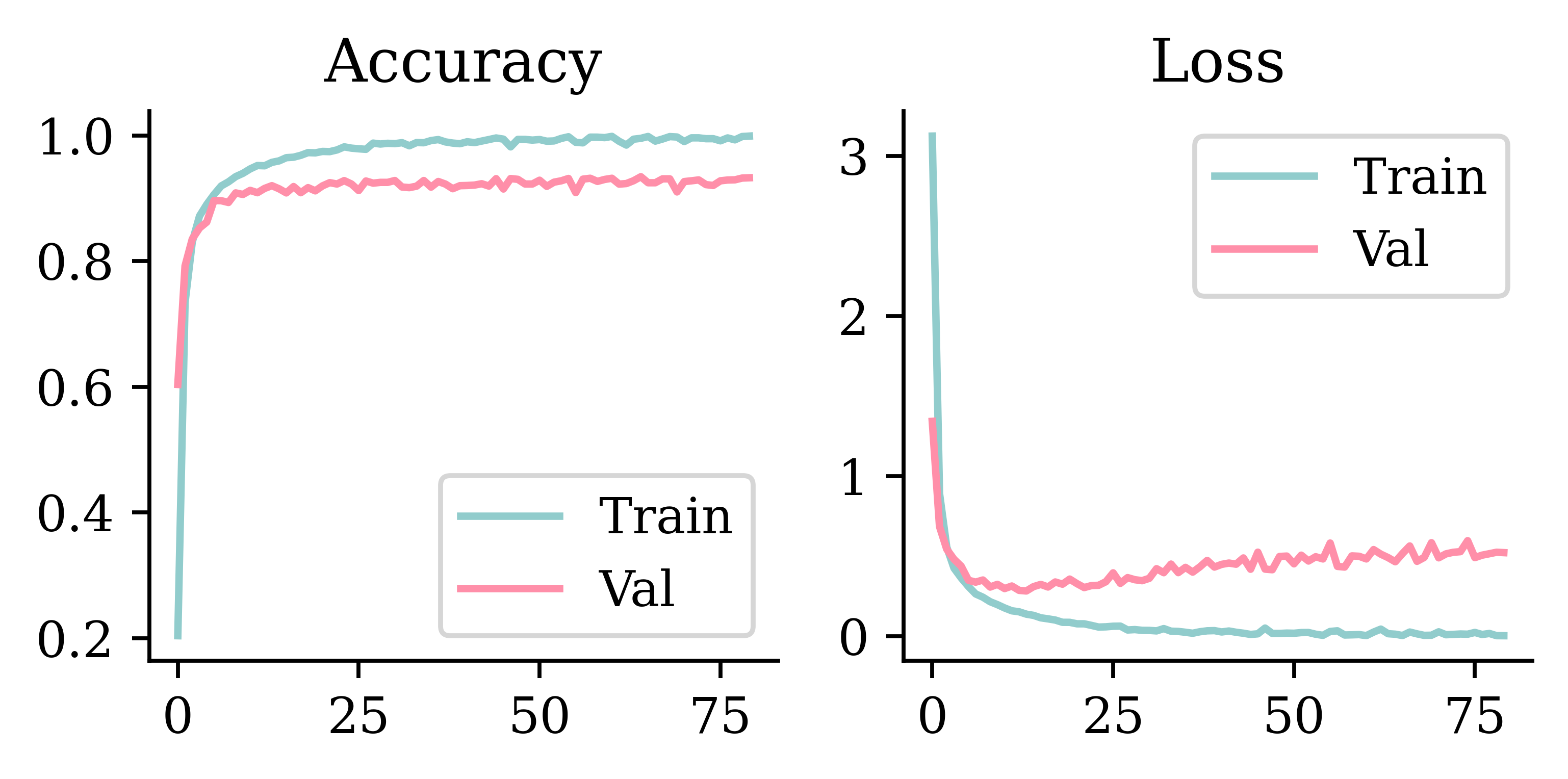

Look at the metrics

print(model.evaluate(X_train, y_train, verbose=0))
print(model.evaluate(X_val, y_val, verbose=0))

[0.0042258091270923615, 0.9987967610359192, 1.0]
[0.46650248765945435, 0.9343371391296387, 0.9953430891036987]

loss_value, accuracy, top5_accuracy = model.evaluate(X_test, y_test, verbose=0)
print(f"Test Loss: {loss_value:.4f}")
print(f"Test Accuracy: {accuracy:.4f}")
print(f"Test Top 5 Accuracy: {top5_accuracy:.4f}")

Test Loss: 0.9513
Test Accuracy: 0.8850
Test Top 5 Accuracy: 0.9875

Predict on the test set

Running model.predict(X_test[0], verbose=0) would crash. Why?

print(X_test[0].shape)
print(X_test[0][np.newaxis, :].shape)
print(X_test[[0]].shape)

(80, 60, 1)
(1, 80, 60, 1)
(1, 80, 60, 1)

Make sure to check the shape of your data to ensure the right inputs to the functions.

model.predict(X_test[[0]], verbose=0)

array([[  39.32,  -42.6 ,  -76.12,  -46.71,  -15.65,  -21.84,  -80.2 ,
         -66.93,  -10.67,    0.46,  -30.95,  -42.12,  -40.14,  -48.4 ,
         -16.2 ,   -3.83,  -17.33,   25.23,   -6.01,  -48.1 ,  -52.31,
         -55.88, -112.03,  -40.44,  -27.87,  -36.71,  -38.15,   -9.84,
          -7.32,  -22.5 ,   -8.18,  -25.79,  -33.83,   10.17,  -27.51,
         -28.83,  -56.86,  -40.7 ,  -40.01,  -40.38,  -51.93,   -8.63,
          -9.4 ,   -0.41,   -2.17,   -8.25,  -19.06,  -11.19,  -74.19,
         -60.56,  -50.35,  -16.09,  -80.93,  -25.66,  -41.95]],
      dtype=float32)

Because we don’t have the softmax activation function, the predicted values don’t directly represent the probabilities (not between 0 and 1). However, the predicted values are ordered according to their respective implied probabilities. In other words, the category with the highest predicted value is the category with the highest implied probability.

Predict on the test set II

model.predict(X_test[[0]], verbose=0).argmax()

np.int64(0)

class_names[model.predict(X_test[[0]], verbose=0).argmax()]

'东'

plt.imshow(X_test[0], cmap="gray");

The predicted category appears to be correct.

Take a look at the failure cases

Code

def plot_failed_predictions(X, y, class_names, max_errors = 20,
            num_rows = 2, num_cols = 5, title_font=CHINESE_FONT):
    plt.figure(figsize=(num_cols * 2, num_rows * 2))
    errors = 0
    y_pred = model.predict(X, verbose=0)
    y_pred_classes = y_pred.argmax(axis=1)
    y_pred_probs = keras.ops.convert_to_numpy(keras.ops.softmax(y_pred)).max(axis=1)
    for i in range(len(y_pred)):
        if errors >= min(max_errors, num_rows * num_cols):
            break
        if y_pred_classes[i] != y[i]:
            plt.subplot(num_rows, num_cols, errors + 1)
            plt.imshow(X[i], cmap="gray")
            true_class = class_names[y[i]]
            pred_class = class_names[y_pred_classes[i]]
            conf = y_pred_probs[i]
            msg = f"{true_class} not {pred_class} ({conf*100:.0f}%)"
            plt.title(msg, fontproperties=title_font)
            plt.axis("off")
            errors += 1

plot_failed_predictions(X_test, y_test, class_names)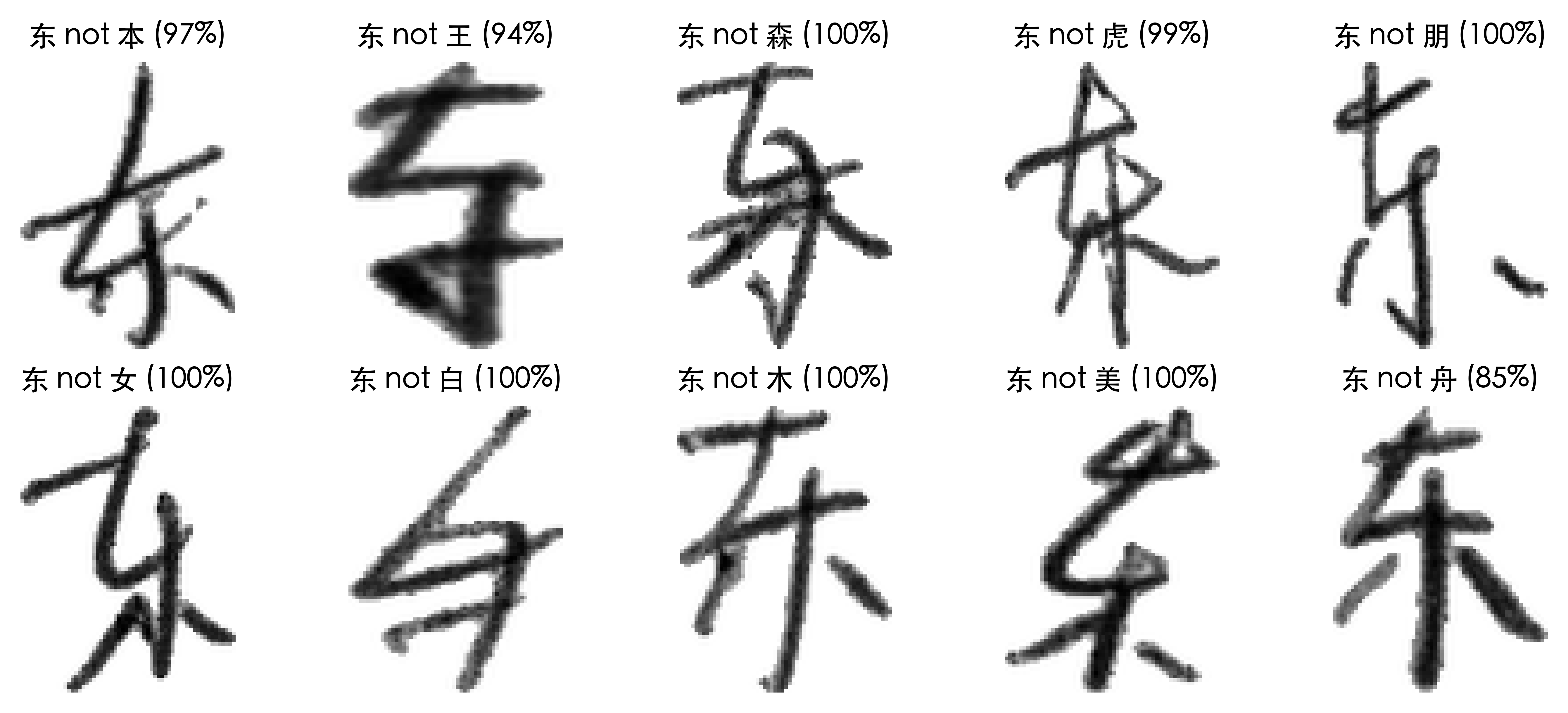

By looking at the failure cases, we can ask ourselves:

Was any of the data mislabeled?
Are there common patterns in the failure cases? E.g. Two different characters that look similar

Confidence of predictions

1y_log = model.predict(X_test, verbose=0)
2y_pred = keras.ops.convert_to_numpy(keras.activations.softmax(y_log))
3y_pred_class = np.argmax(y_pred, axis=1)
4y_pred_prob = y_pred[np.arange(y_pred.shape[0]), y_pred_class]

confidence_when_correct = y_pred_prob[y_pred_class == y_test]
5confidence_when_wrong = y_pred_prob[y_pred_class != y_test]

1: Make predictions on the test set
2: Convert the predictions to probabilities [0,1] using softmax activation function
3: Extract the category with the highest probability (the prediction’s best guess)
4: Extract the probability of the above category
5: Split the probabilities between correct and incorrect guesses

plt.hist(confidence_when_correct);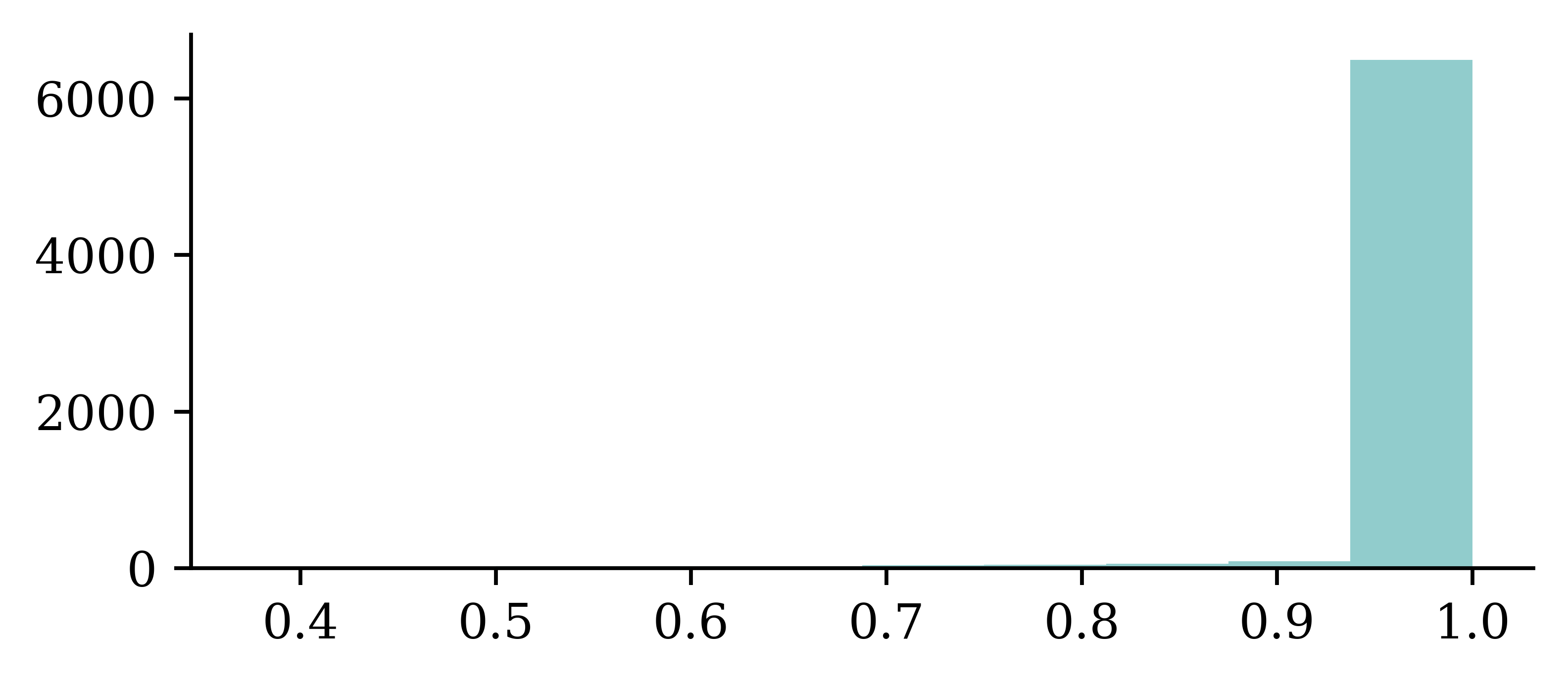

plt.hist(confidence_when_wrong);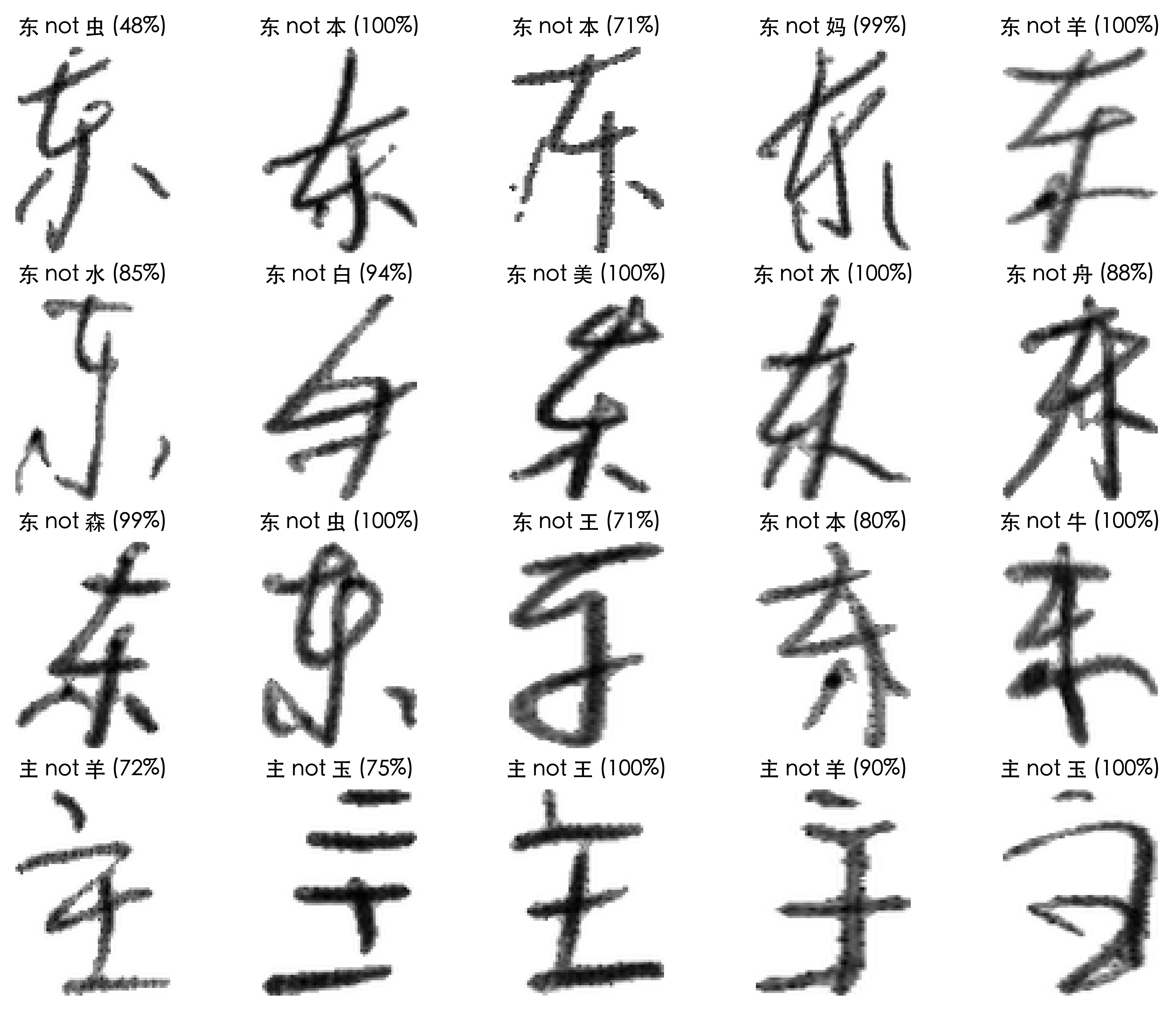

For correct guesses, almost all of them were at least 90% confident. For incorrect guesses, the guesses were less confident on average, but most of the guesses were still at least 90% confident.

Hyperparameter Optimisation

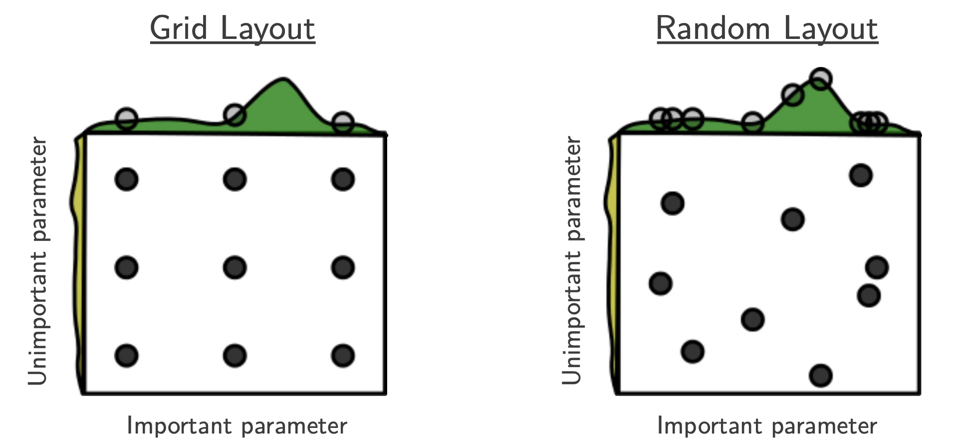
How do we pick the best hyperparameters?

Make a range potential values for hyperparameter, and try many combinations of them.

“hyper-parameter optimization should be regarded as a formal outer loop in the learning process”

— Bergstra et al. (2011, p. 1).

“HPO faces several challenges which make it a hard problem in practice:

Function evaluations can be extremely expensive for large models (e.g., in deep learning), complex machine learning pipelines, or large datesets.

The configuration space is often complex (comprising a mix of continuous, categorical and conditional hyperparameters) and high-dimensional. Furthermore, it is not always clear which of an algorithm’s hyperparameters need to be optimized, and in which ranges.

We usually don’t have access to a gradient of the loss function with respect to the hyperparameters.”

— Feurer & Hutter (2019, p. 4)

Could we just try every combination?

This technique, called grid search, would be too slow. Better to take random selections.

Random search is safer to use than grid search. .

Optuna

def objective(trial):
1    keras.utils.set_random_seed(trial.number)
    model = Sequential()
    model.add(Dense(
        trial.suggest_categorical("neurons", [4, 8, 16, 32, 64, 128, 256]),
        activation=trial.suggest_categorical("activation",
            ["relu", "leaky_relu", "tanh"]),
    ))
    model.add(Dense(1, activation="exponential"))

    learning_rate = trial.suggest_float("lr", 1e-4, 1e-2, log=True)
    opt = keras.optimizers.Adam(learning_rate=learning_rate)
    model.compile(optimizer=opt, loss="poisson")

    es = EarlyStopping(patience=3, restore_best_weights=True)
    model.fit(X_train_sc, y_train, epochs=100, batch_size=256,
        callbacks=[es], validation_data=(X_val_sc, y_val), verbose=0)

    return model.evaluate(X_val_sc, y_val, verbose=0)

1: Seeding with the trial number makes each model’s weight initialisation and mini-batch shuffling reproducible, so the winning trial can be rebuilt exactly afterwards.

The hyperparameters we are tuning are:

The number of neurons in each hidden layer
The activation functions for the hidden layers
The learning rate for the Adam optimiser

We give the model a few choices for the first two (the learning rate is continuous). Note that with Optuna, the objective function handles the entire training loop and returns the validation loss. Optuna then uses this to decide which hyperparameters to try next.

Do a random search

sampler = optuna.samplers.RandomSampler(seed=123)
study = optuna.create_study(direction="minimize", sampler=sampler)

study.optimize(objective, n_trials=10)

[I 2026-06-15 10:39:14,852] A new study created in memory with name: no-name-0f385609-a748-4bc0-8e8d-e2d0f7731ccd

[I 2026-06-15 10:39:20,868] Trial 0 finished with value: 0.31880027055740356 and parameters: {'neurons': 256, 'activation': 'relu', 'lr': 0.00048568650020512866}. Best is trial 0 with value: 0.31880027055740356.

[I 2026-06-15 10:39:23,115] Trial 1 finished with value: 0.322916716337204 and parameters: {'neurons': 64, 'activation': 'tanh', 'lr': 0.004998774988536159}. Best is trial 0 with value: 0.31880027055740356.

[I 2026-06-15 10:39:29,468] Trial 2 finished with value: 0.34097015857696533 and parameters: {'neurons': 4, 'activation': 'relu', 'lr': 0.0007273199943087333}. Best is trial 0 with value: 0.31880027055740356.

[I 2026-06-15 10:39:33,718] Trial 3 finished with value: 0.32092881202697754 and parameters: {'neurons': 128, 'activation': 'relu', 'lr': 0.0006755421067424912}. Best is trial 0 with value: 0.31880027055740356.

[I 2026-06-15 10:39:40,156] Trial 4 finished with value: 0.3249039947986603 and parameters: {'neurons': 32, 'activation': 'relu', 'lr': 0.00048476099425358564}. Best is trial 0 with value: 0.31880027055740356.

[I 2026-06-15 10:39:46,438] Trial 5 finished with value: 0.3413579761981964 and parameters: {'neurons': 32, 'activation': 'tanh', 'lr': 0.00014668644271977285}. Best is trial 0 with value: 0.31880027055740356.

[I 2026-06-15 10:39:48,134] Trial 6 finished with value: 0.3263881802558899 and parameters: {'neurons': 128, 'activation': 'relu', 'lr': 0.0012988840529683243}. Best is trial 0 with value: 0.31880027055740356.

[I 2026-06-15 10:39:54,556] Trial 7 finished with value: 24.464731216430664 and parameters: {'neurons': 16, 'activation': 'relu', 'lr': 0.0001222314398350804}. Best is trial 0 with value: 0.31880027055740356.

[I 2026-06-15 10:40:00,930] Trial 8 finished with value: 0.5315024852752686 and parameters: {'neurons': 32, 'activation': 'relu', 'lr': 0.0003031878514851357}. Best is trial 0 with value: 0.31880027055740356.

[I 2026-06-15 10:40:07,390] Trial 9 finished with value: 0.33647409081459045 and parameters: {'neurons': 16, 'activation': 'tanh', 'lr': 0.0005884040083055758}. Best is trial 0 with value: 0.31880027055740356.

print(f"Best value: {study.best_trial.value:.4f}")
print(f"Best params:")
for k, v in study.best_trial.params.items():
    print(f"  {k}: {v}")

Best value: 0.3188
Best params:
  neurons: 256
  activation: relu
  lr: 0.00048568650020512866

The model runs through 10 random combinations of the hyperparameters and returns the one where the loss on the validation set is minimised.

Recover the winning model

Because each trial seeded itself with its own trial number, we can rebuild the exact winning model from its saved parameters — no need to store the trained weights.

p = study.best_trial.params
keras.utils.set_random_seed(study.best_trial.number)

best_model = Sequential([
    Dense(p["neurons"], activation=p["activation"]),
    Dense(1, activation="exponential"),
])
best_model.compile(optimizer=keras.optimizers.Adam(p["lr"]), loss="poisson")

es = EarlyStopping(patience=3, restore_best_weights=True)
best_model.fit(X_train_sc, y_train, epochs=100, batch_size=256,
    callbacks=[es], validation_data=(X_val_sc, y_val), verbose=0)

print(f"Rebuilt loss: {best_model.evaluate(X_val_sc, y_val, verbose=0):.4f}")
print(f"Tuning best:  {study.best_trial.value:.4f}")

Rebuilt loss: 0.3188
Tuning best:  0.3188

The rebuilt model’s validation loss matches the value found during tuning, confirming we have recovered the same model. The seed must be set at the top of the function — before the model is built and trained — since it controls both the weight initialisation and the order the training data is shuffled in.

Tune layers separately

def objective(trial):
    keras.utils.set_random_seed(trial.number)
    model = Sequential()

    for i in range(trial.suggest_int("numHiddenLayers", 1, 3)):
        model.add(Dense(
            trial.suggest_categorical(f"neurons_{i}", [8, 16, 32, 64]),
            activation="relu"))
    model.add(Dense(1, activation="exponential"))

    opt = keras.optimizers.Adam(learning_rate=0.0005)
    model.compile(optimizer=opt, loss="poisson")

    es = EarlyStopping(patience=3, restore_best_weights=True)
    model.fit(X_train_sc, y_train, epochs=100, batch_size=256,
        callbacks=[es], validation_data=(X_val_sc, y_val), verbose=0)

    return model.evaluate(X_val_sc, y_val, verbose=0)

This time, we let the number of neurons in each hidden layer be tuned separately. For this example we are not tuning the activation functions or the learning rate.

Do a Bayesian search

1sampler = optuna.samplers.TPESampler(seed=123, n_startup_trials=5)
study = optuna.create_study(direction="minimize", sampler=sampler)

study.optimize(objective, n_trials=10)

1: Optuna uses a Tree-structured Parzen Estimator (TPE) by default, which is a Bayesian method. Passing a seed makes the search reproducible. The first n_startup_trials are sampled randomly to seed the model (the default is 10); we lower it to 5 so the later trials are actually chosen by TPE.

[I 2026-06-15 10:40:13,412] A new study created in memory with name: no-name-4a98a603-0170-47da-9b88-c8ac8ed9ebba

[I 2026-06-15 10:40:20,019] Trial 0 finished with value: 0.31632715463638306 and parameters: {'numHiddenLayers': 3, 'neurons_0': 64, 'neurons_1': 16, 'neurons_2': 32}. Best is trial 0 with value: 0.31632715463638306.

[I 2026-06-15 10:40:26,458] Trial 1 finished with value: 0.3395172357559204 and parameters: {'numHiddenLayers': 1, 'neurons_0': 16}. Best is trial 0 with value: 0.31632715463638306.

[I 2026-06-15 10:40:32,772] Trial 2 finished with value: 0.32005345821380615 and parameters: {'numHiddenLayers': 2, 'neurons_0': 32, 'neurons_1': 16}. Best is trial 0 with value: 0.31632715463638306.

[I 2026-06-15 10:40:39,187] Trial 3 finished with value: 0.33305951952934265 and parameters: {'numHiddenLayers': 1, 'neurons_0': 16}. Best is trial 0 with value: 0.31632715463638306.

[I 2026-06-15 10:40:46,913] Trial 4 finished with value: 0.3474620282649994 and parameters: {'numHiddenLayers': 2, 'neurons_0': 8, 'neurons_1': 16}. Best is trial 0 with value: 0.31632715463638306.

[I 2026-06-15 10:40:48,801] Trial 5 finished with value: 0.32650327682495117 and parameters: {'numHiddenLayers': 3, 'neurons_0': 64, 'neurons_1': 64, 'neurons_2': 32}. Best is trial 0 with value: 0.31632715463638306.

[I 2026-06-15 10:40:55,641] Trial 6 finished with value: 0.31397563219070435 and parameters: {'numHiddenLayers': 3, 'neurons_0': 64, 'neurons_1': 32, 'neurons_2': 32}. Best is trial 6 with value: 0.31397563219070435.

[I 2026-06-15 10:40:59,440] Trial 7 finished with value: 0.31934303045272827 and parameters: {'numHiddenLayers': 3, 'neurons_0': 64, 'neurons_1': 32, 'neurons_2': 64}. Best is trial 6 with value: 0.31397563219070435.

[I 2026-06-15 10:41:03,989] Trial 8 finished with value: 0.32798051834106445 and parameters: {'numHiddenLayers': 3, 'neurons_0': 32, 'neurons_1': 32, 'neurons_2': 16}. Best is trial 6 with value: 0.31397563219070435.

[I 2026-06-15 10:41:11,233] Trial 9 finished with value: 0.3356526494026184 and parameters: {'numHiddenLayers': 2, 'neurons_0': 8, 'neurons_1': 8}. Best is trial 6 with value: 0.31397563219070435.

print(f"Best value: {study.best_trial.value:.4f}")
print(f"Best params:")
for k, v in study.best_trial.params.items():
    print(f"  {k}: {v}")

Best value: 0.3140
Best params:
  numHiddenLayers: 3
  neurons_0: 64
  neurons_1: 32
  neurons_2: 32

Tip

Neural networks are sensitive to their random initialisation: a hyperparameter combination that looks good (or bad) on a single run might just have been lucky. A more robust approach is to train 3–5 models with the same hyperparameters but different random seeds, and average the validation loss — selecting architectures that perform well and reliably.

Bayesian search is not purely random, and updates its beliefs about the optimal hyperparameter values based on past models. Bayesian search balances exploration of new hyperparameter values and exploitation of the values that are expected to be optimal. Optuna’s default sampler is the Tree-structured Parzen Estimator (TPE), which is a Bayesian optimization algorithm. Passing a seed to the sampler ensures the same sequence of hyperparameters is tried each time.

In the objective function, instead of returning the loss from a single fit, you would loop over a few seeds, refit each time, and return the mean validation loss. This is slower but gives you much more confidence that the chosen hyperparameters are genuinely good rather than a fluke.

Transfer Learning

Demo: Object classification

How are these classification models so accurate?

“… these models use a technique called transfer learning. There’s a pretrained neural network, and when you create your own classes, you can sort of picture that your classes are becoming the last layer or step of the neural net. Specifically, both the image and pose models are learning off of pretrained mobilenet models …”

Transfer learned model

model_file = "converted_keras/keras_model.h5"
model = keras.models.load_model(model_file)

model.layers[0].layers[0].layers

[<InputLayer name=input_1, built=True>,
<ZeroPadding2D name=Conv1_pad, built=True>,
<Conv2D name=Conv1, built=True>,
<BatchNormalization name=bn_Conv1, built=True>,
<ReLU name=Conv1_relu, built=True>,
<DepthwiseConv2D name=expanded_conv_depthwise, built=True>,
<BatchNormalization name=expanded_conv_depthwise_BN, built=True>,
<ReLU name=expanded_conv_depthwise_relu, built=True>,
<Conv2D name=expanded_conv_project, built=True>,
<BatchNormalization name=expanded_conv_project_BN, built=True>,
<Conv2D name=block_1_expand, built=True>,
<BatchNormalization name=block_1_expand_BN, built=True>,
<ReLU name=block_1_expand_relu, built=True>,
<ZeroPadding2D name=block_1_pad, built=True>,
<DepthwiseConv2D name=block_1_depthwise, built=True>,
<BatchNormalization name=block_1_depthwise_BN, built=True>,
<ReLU name=block_1_depthwise_relu, built=True>,
<Conv2D name=block_1_project, built=True>,
<BatchNormalization name=block_1_project_BN, built=True>,
<Conv2D name=block_2_expand, built=True>,
<BatchNormalization name=block_2_expand_BN, built=True>,
<ReLU name=block_2_expand_relu, built=True>,
<DepthwiseConv2D name=block_2_depthwise, built=True>,
<BatchNormalization name=block_2_depthwise_BN, built=True>,
<ReLU name=block_2_depthwise_relu, built=True>,
<Conv2D name=block_2_project, built=True>,
<BatchNormalization name=block_2_project_BN, built=True>,
<Add name=block_2_add, built=True>,
<Conv2D name=block_3_expand, built=True>,
<BatchNormalization name=block_3_expand_BN, built=True>,
<ReLU name=block_3_expand_relu, built=True>,
<ZeroPadding2D name=block_3_pad, built=True>,
<DepthwiseConv2D name=block_3_depthwise, built=True>,
<BatchNormalization name=block_3_depthwise_BN, built=True>,
<ReLU name=block_3_depthwise_relu, built=True>,
<Conv2D name=block_3_project, built=True>,
<BatchNormalization name=block_3_project_BN, built=True>,
<Conv2D name=block_4_expand, built=True>,
<BatchNormalization name=block_4_expand_BN, built=True>,
<ReLU name=block_4_expand_relu, built=True>,
<DepthwiseConv2D name=block_4_depthwise, built=True>,
<BatchNormalization name=block_4_depthwise_BN, built=True>,
<ReLU name=block_4_depthwise_relu, built=True>,
<Conv2D name=block_4_project, built=True>,
<BatchNormalization name=block_4_project_BN, built=True>,
<Add name=block_4_add, built=True>,
<Conv2D name=block_5_expand, built=True>,
<BatchNormalization name=block_5_expand_BN, built=True>,
<ReLU name=block_5_expand_relu, built=True>,
<DepthwiseConv2D name=block_5_depthwise, built=True>,
<BatchNormalization name=block_5_depthwise_BN, built=True>,
<ReLU name=block_5_depthwise_relu, built=True>,
<Conv2D name=block_5_project, built=True>,
<BatchNormalization name=block_5_project_BN, built=True>,
<Add name=block_5_add, built=True>,
<Conv2D name=block_6_expand, built=True>,
<BatchNormalization name=block_6_expand_BN, built=True>,
<ReLU name=block_6_expand_relu, built=True>,
<ZeroPadding2D name=block_6_pad, built=True>,
<DepthwiseConv2D name=block_6_depthwise, built=True>,
<BatchNormalization name=block_6_depthwise_BN, built=True>,
<ReLU name=block_6_depthwise_relu, built=True>,
<Conv2D name=block_6_project, built=True>,
<BatchNormalization name=block_6_project_BN, built=True>,
<Conv2D name=block_7_expand, built=True>,
<BatchNormalization name=block_7_expand_BN, built=True>,
<ReLU name=block_7_expand_relu, built=True>,
<DepthwiseConv2D name=block_7_depthwise, built=True>,
<BatchNormalization name=block_7_depthwise_BN, built=True>,
<ReLU name=block_7_depthwise_relu, built=True>,
<Conv2D name=block_7_project, built=True>,
<BatchNormalization name=block_7_project_BN, built=True>,
<Add name=block_7_add, built=True>,
<Conv2D name=block_8_expand, built=True>,
<BatchNormalization name=block_8_expand_BN, built=True>,
<ReLU name=block_8_expand_relu, built=True>,
<DepthwiseConv2D name=block_8_depthwise, built=True>,
<BatchNormalization name=block_8_depthwise_BN, built=True>,
<ReLU name=block_8_depthwise_relu, built=True>,
<Conv2D name=block_8_project, built=True>,
<BatchNormalization name=block_8_project_BN, built=True>,
<Add name=block_8_add, built=True>,
<Conv2D name=block_9_expand, built=True>,
<BatchNormalization name=block_9_expand_BN, built=True>,
<ReLU name=block_9_expand_relu, built=True>,
<DepthwiseConv2D name=block_9_depthwise, built=True>,
<BatchNormalization name=block_9_depthwise_BN, built=True>,
<ReLU name=block_9_depthwise_relu, built=True>,
<Conv2D name=block_9_project, built=True>,
<BatchNormalization name=block_9_project_BN, built=True>,
<Add name=block_9_add, built=True>,
<Conv2D name=block_10_expand, built=True>,
<BatchNormalization name=block_10_expand_BN, built=True>,
<ReLU name=block_10_expand_relu, built=True>,
<DepthwiseConv2D name=block_10_depthwise, built=True>,
<BatchNormalization name=block_10_depthwise_BN, built=True>,
<ReLU name=block_10_depthwise_relu, built=True>,
<Conv2D name=block_10_project, built=True>,
<BatchNormalization name=block_10_project_BN, built=True>,
<Conv2D name=block_11_expand, built=True>,
<BatchNormalization name=block_11_expand_BN, built=True>,
<ReLU name=block_11_expand_relu, built=True>,
<DepthwiseConv2D name=block_11_depthwise, built=True>,
<BatchNormalization name=block_11_depthwise_BN, built=True>,
<ReLU name=block_11_depthwise_relu, built=True>,
<Conv2D name=block_11_project, built=True>,
<BatchNormalization name=block_11_project_BN, built=True>,
<Add name=block_11_add, built=True>,
<Conv2D name=block_12_expand, built=True>,
<BatchNormalization name=block_12_expand_BN, built=True>,
<ReLU name=block_12_expand_relu, built=True>,
<DepthwiseConv2D name=block_12_depthwise, built=True>,
<BatchNormalization name=block_12_depthwise_BN, built=True>,
<ReLU name=block_12_depthwise_relu, built=True>,
<Conv2D name=block_12_project, built=True>,
<BatchNormalization name=block_12_project_BN, built=True>,
<Add name=block_12_add, built=True>,
<Conv2D name=block_13_expand, built=True>,
<BatchNormalization name=block_13_expand_BN, built=True>,
<ReLU name=block_13_expand_relu, built=True>,
<ZeroPadding2D name=block_13_pad, built=True>,
<DepthwiseConv2D name=block_13_depthwise, built=True>,
<BatchNormalization name=block_13_depthwise_BN, built=True>,
<ReLU name=block_13_depthwise_relu, built=True>,
<Conv2D name=block_13_project, built=True>,
<BatchNormalization name=block_13_project_BN, built=True>,
<Conv2D name=block_14_expand, built=True>,
<BatchNormalization name=block_14_expand_BN, built=True>,
<ReLU name=block_14_expand_relu, built=True>,
<DepthwiseConv2D name=block_14_depthwise, built=True>,
<BatchNormalization name=block_14_depthwise_BN, built=True>,
<ReLU name=block_14_depthwise_relu, built=True>,
<Conv2D name=block_14_project, built=True>,
<BatchNormalization name=block_14_project_BN, built=True>,
<Add name=block_14_add, built=True>,
<Conv2D name=block_15_expand, built=True>,
<BatchNormalization name=block_15_expand_BN, built=True>,
<ReLU name=block_15_expand_relu, built=True>,
<DepthwiseConv2D name=block_15_depthwise, built=True>,
<BatchNormalization name=block_15_depthwise_BN, built=True>,
<ReLU name=block_15_depthwise_relu, built=True>,
<Conv2D name=block_15_project, built=True>,
<BatchNormalization name=block_15_project_BN, built=True>,
<Add name=block_15_add, built=True>,
<Conv2D name=block_16_expand, built=True>,
<BatchNormalization name=block_16_expand_BN, built=True>,
<ReLU name=block_16_expand_relu, built=True>,
<DepthwiseConv2D name=block_16_depthwise, built=True>,
<BatchNormalization name=block_16_depthwise_BN, built=True>,
<ReLU name=block_16_depthwise_relu, built=True>,
<Conv2D name=block_16_project, built=True>,
<BatchNormalization name=block_16_project_BN, built=True>,
<Conv2D name=Conv_1, built=True>,
<BatchNormalization name=Conv_1_bn, built=True>,
<ReLU name=out_relu, built=True>]

len(model.layers[0].layers[0].layers)

The model has 155 layers.

The original pretrained model

Transfer learning

# Pull in the base model we are transferring from.
base_model = keras.applications.Xception(
    weights="imagenet",  # Load weights pre-trained on ImageNet.
    input_shape=(150, 150, 3),
    include_top=False,
)  # Discard the ImageNet classifier at the top.

# Tell it not to update its weights.
base_model.trainable = False

# Make our new model on top of the base model.
inputs = Input(shape=(150, 150, 3))
x = base_model(inputs, training=False)
x = GlobalAveragePooling2D()(x)
outputs = Dense(1)(x)
model = Model(inputs, outputs)

# Compile and fit on our data.
model.compile(
    optimizer=keras.optimizers.Adam(),
    loss=keras.losses.BinaryCrossentropy(from_logits=True),
    metrics=[keras.metrics.BinaryAccuracy()],
)
model.fit(new_dataset, epochs=2, callbacks=..., validation_data=...)

Fine-tuning

# Unfreeze the base model
base_model.trainable = True

# It's important to recompile your model after you make any changes
# to the `trainable` attribute of any inner layer, so that your changes
# are take into account
model.compile(
    optimizer=keras.optimizers.Adam(1e-5),  # Very low learning rate
    loss=keras.losses.BinaryCrossentropy(from_logits=True),
    metrics=[keras.metrics.BinaryAccuracy()],
)

# Train end-to-end. Be careful to stop before you overfit!
model.fit(new_dataset, epochs=1, callbacks=..., validation_data=...)

Caution

Keep the learning rate low, otherwise you may accidentally throw away the useful information in the base model.

References

Package Versions

from watermark import watermark
print(watermark(python=True, packages="keras,matplotlib,numpy,pandas,seaborn,scipy,torch"))

Python implementation: CPython
Python version       : 3.14.5
IPython version      : 9.13.0

keras     : 3.14.1
matplotlib: 3.10.9
numpy     : 2.4.4
pandas    : 3.0.2
seaborn   : 0.13.2
scipy     : 1.17.1
torch     : 2.11.0

Glossary

AlexNet
channels
computer vision
convolutional layer
convolutional network
filter
ImageNet challenge
fine-tuning

flatten layer
kernel
max pooling
MNIST
stride
tensor (rank)
transfer learning

References

Bergstra, J., Bardenet, R., Bengio, Y., & Kégl, B. (2011). Algorithms for hyper-parameter optimization. Advances in Neural Information Processing Systems, 24.

Bergstra, J., & Bengio, Y. (2012). Random search for hyper-parameter optimization. Journal of Machine Learning Research, 13(2).

Feurer, M., & Hutter, F. (2019). Hyperparameter optimization. In Automated machine learning: Methods, systems, challenges (pp. 3–33). Springer.

Géron, A. (2022). Hands-on machine learning with Scikit-Learn, Keras, and TensorFlow (3rd ed.). O’Reilly Media.

Glassner, A. (2021). Deep learning: A visual approach. No Starch Press.

Goodfellow, I. J., Bulatov, Y., Ibarz, J., Arnoud, S., & Shet, V. (2014). Multi-digit number recognition from street view imagery using deep convolutional neural networks. arXiv Preprint arXiv:1312.6082.

Liu, C.-L., Yin, F., Wang, D.-H., & Wang, Q.-F. (2011). CASIA online and offline chinese handwriting databases. 2011 International Conference on Document Analysis and Recognition, 37–41.