Python for Data Science

ACTL3143 & ACTL5111 Deep Learning for Actuaries

Author

Patrick Laub

Preliminary notes

Readings for this topic:

Week	Readings (ACTL3142 Revision)
1	James et al. (2021): Chapter 2, Sections 3.1, 3.2, and 5.1.1
2	James et al. (2021): Section 3.3.1, 4.1, 4.2, 4.3

For ACTL3143 students, these slides are mostly a revision of ACTL3142 concepts but using Python instead of R.

For ACTL5111 students, if you have not taken ACTL5110, you need to self-study any surprising concepts in these slides ASAP.

Introduction to Statistical Learning with R Python

Machine learning workflow

An entire ML project

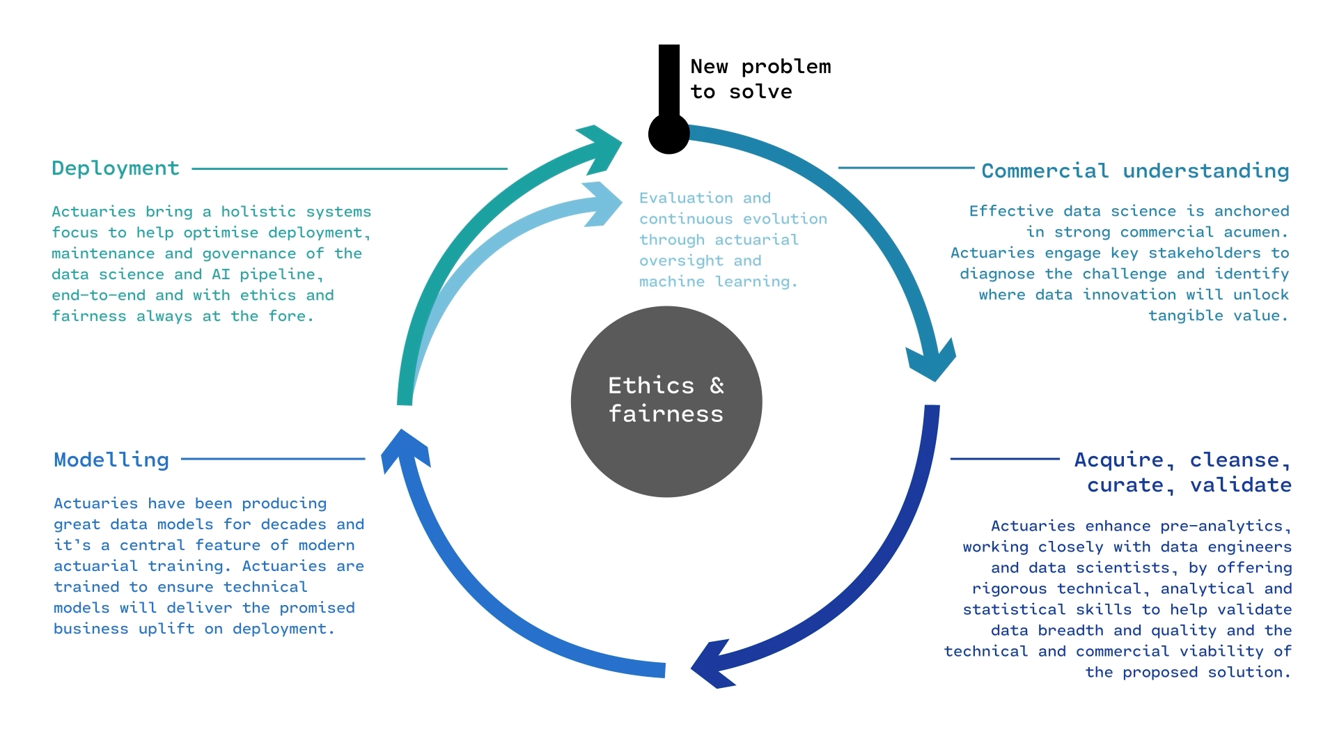
The course focuses more on the modelling part of the life cycle.

Questions to answer in ML project

You fit a few models to the training set, then ask:

(Selection) Which of these models is the best?
(Future Performance) How good should we expect the final model to be on unseen data?

Illustration of a typical training/test split.

Validation set approach

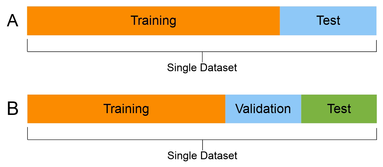
For each model, fit it to the training set.
Compute the error for each model on the validation set.
Select the model with the lowest validation error.
Compute the error of the final model on the test set.

Read Section 5.1.1 of James et al. (2021) for details.

You should have seen split A in your previous courses. In those courses, split A is used, and then cross-validation is performed to fit the hyperparameters. In the case of NNs, it is much more common to split the dataset into training, validation and test (split B).

Data science packages

Imports for these slides

import numpy as np
import pandas as pd
import matplotlib.pyplot as plt

from sklearn.datasets import fetch_california_housing
from sklearn.linear_model import LinearRegression, LogisticRegression, PoissonRegressor
from sklearn.metrics import mean_squared_error
from sklearn.model_selection import train_test_split
from sklearn.preprocessing import StandardScaler
from sklearn.tree import DecisionTreeClassifier, plot_tree

Numpy for matrices

Numpy is Python’s standard approach for any low-level numerical mathematics tasks (matrix processing, linear algebra)

a = np.array([1, 2, 3, 4])
a.mean(), a.std()

(np.float64(2.5), np.float64(1.118033988749895))

a * 2 + 1 # vectorised arithmetic

array([3, 5, 7, 9])

M = np.arange(6).reshape(2, 3)
M

array([[0, 1, 2],
       [3, 4, 5]])

M.shape, M.sum(axis=0)

((2, 3), array([3, 5, 7]))

Travis Oliphant, creator of Numpy (and Scipy). Now >2K contributors, ~450K LOC (C), 19B installs (Open Hub and ClickPy)

Also has random number generation functionality

rng = np.random.default_rng(0)
x = rng.normal(size=200)
y = 2 * x + rng.normal(size=200)

Pandas for DataFrames

Used for tabular data: loading, cleaning, processing, saving

df = pd.DataFrame({
    "age": [25, 32, 41, 28, 36],
    "salary": [45_000, 65_000, 80_000, 55_000, 72_000],
})
df.head()

	age	salary
0	25	45000
1	32	65000
2	41	80000
3	28	55000
4	36	72000

Wes McKinney, creator of Pandas. Now >4K contributors, ~475K LOC (Python), 14B installs (Open Hub and ClickPy)

df.shape          # (rows, cols)
df.columns.tolist()

['age', 'salary']

df["age"]         # column
df.iloc[0]        # first row

age          25
salary    45000
Name: 0, dtype: int64

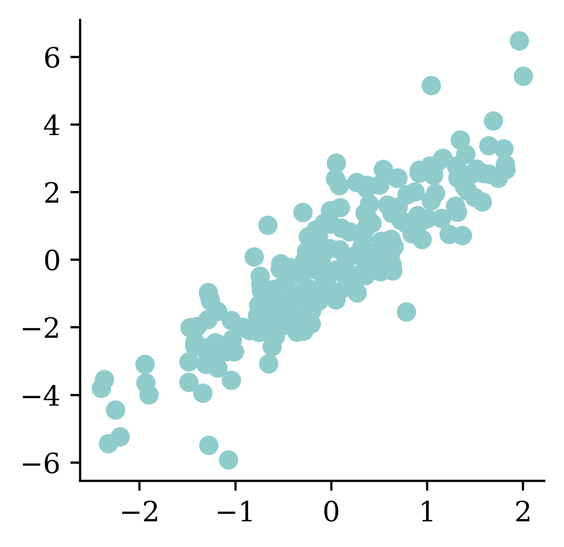
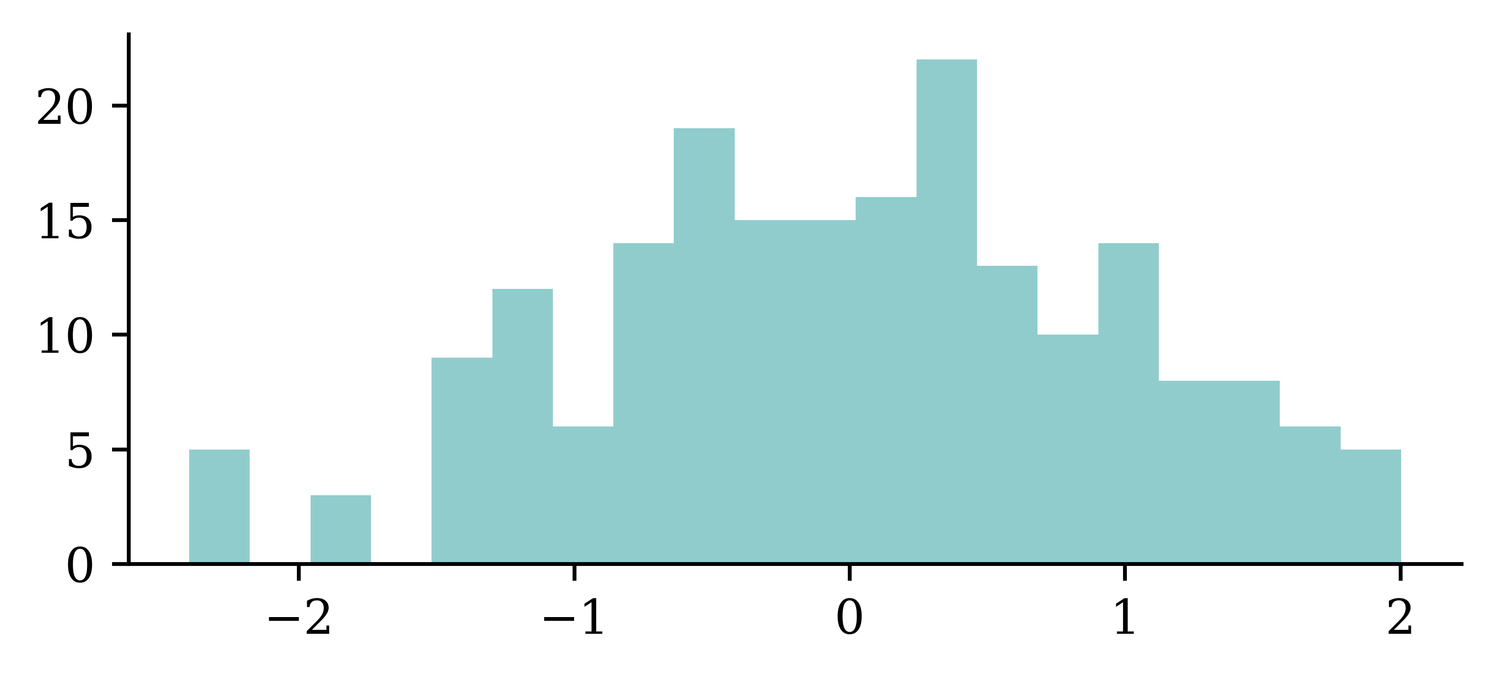
Matplotlib for plots

The traditional way to generate plots; similar (in spirit) to R’s base plot()

plt.figure(figsize=(3, 3))
plt.scatter(x, y);

John D. Hunter (1968–2012), creator of Matplotlib. Now has ~290K LOC (Python), >2K contributors, 4B installs (Open Hub and ClickPy)

plt.hist(x, bins=20);

Scikit-learn for machine learning

Every sklearn estimator has the same three methods:

fit(X, y): learn the parameters of the model
predict(X): apply the model
score(X, y): apply the model and calculate a metric

X = df[["age"]] # [[ ]] gives a 2D DataFrame
y = df["salary"]
model = LinearRegression()
model.fit(X, y)
y_pred = model.predict(X)
print(f"R^2 = {model.score(X, y):.3f}")

R^2 = 0.977

Once you’ve learned this pattern for LinearRegression, you’ve largely learned it for every other model in scikit-learn — LogisticRegression, PoissonRegressor, DecisionTreeClassifier, RandomForestRegressor, and so on all use the same three methods.

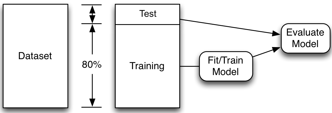
Set aside a fraction for a test set

Off-screen I have loaded up a larger X & y dataset:

print(X.shape, y.shape)

(10000, 4) (10000,)

We can split into train and test sets (in a random but reproducible way):

X_train, X_test, y_train, y_test = train_test_split(X, y, random_state=42)
print(X_train.shape, X_test.shape, y_train.shape, y_test.shape)

(7500, 4) (2500, 4) (7500,) (2500,)

We set aside the test data, assuming it represents new, unseen data. Then we fit many models on the train data and select the one with the lowest train error. Thereafter we assess the performance of that model using the unseen test data.

Note: Compare X_/y_ names, capitals & lowercase.

Split three ways:

Using the same dataset for both validating and testing purposes can result in data leakage: the information from supposedly ‘unseen’ data is now used by the model during its training. This results in a situation where the model is now ‘learning’ from the test data, which could lead to overly optimistic results in the model evaluation stage. That is why it is important to split the data three ways.

1X_main, X_test, y_main, y_test = train_test_split(X, y, test_size=0.2, random_state=1)

# As 0.25 x 0.8 = 0.2
2X_train, X_val, y_train, y_val = train_test_split(X_main, y_main, test_size=0.25, random_state=1)

X_train.shape, X_val.shape, X_test.shape

1: Splits the entire dataset into two parts. Sets aside 20\% of the data as the test set.
2: Splits the first 80\% of the data (X_main and y_main) further into train and validation sets. Sets aside 25\% as the validation set.

((6000, 4), (2000, 4), (2000, 4))

This results in a 60:20:20 three-way split. While this is not a strict rule, it is widely used.

Linear Regression Recap

Single Linear Regression (SLR)

Scenario: use head circumference (mm) to predict age (weeks) of a fetal baby

\boldsymbol{x} = \begin{pmatrix} 105 \\ 120 \\ 110 \\ 117 \\ \end{pmatrix}, \quad \boldsymbol{y} = \begin{pmatrix} 20 \\ 24 \\ 22 \\ 23 \\ \end{pmatrix}, \quad \hat{\boldsymbol{y}} = \begin{pmatrix} 20.3 \\ 24.0 \\ 21.5 \\ 23.2 \\ \end{pmatrix}

\hat{y}(x) = \beta_0 + \beta_1 x

babies = pd.DataFrame({
    "circumference": [105, 120, 110, 117],
    "age": [20, 24, 22, 23],
})
X = babies[["circumference"]]
y = babies["age"]
model = LinearRegression()
model.fit(X, y)
model.predict(X)

array([20.28, 23.97, 21.51, 23.24])

Mean squared error

\boldsymbol{y} = \begin{pmatrix} 20 \\ 24 \\ 22 \\ 23 \\ \end{pmatrix}, \quad \hat{\boldsymbol{y}} = \begin{pmatrix} 20.3 \\ 24.0 \\ 21.5 \\ 23.2 \\ \end{pmatrix}, \quad \boldsymbol{y} - \hat{\boldsymbol{y}} = \begin{pmatrix} -0.3 \\ 0 \\ 0.5 \\ -0.2 \\ \end{pmatrix}.

Code

predicted_age = model.predict(X)

x = babies["circumference"].to_numpy()
y = babies["age"].to_numpy()
yhat = predicted_age
error = np.abs(y - yhat)
mse = np.mean(error ** 2)

fig, ax = plt.subplots(figsize=(8, 2), dpi=300)
ax.scatter(x, y, color="black", zorder=3)
order = np.argsort(x)
ax.plot(x[order], yhat[order], color="black")
for xi, yi, yhi, ei in zip(x, y, yhat, error):
    ax.plot([xi, xi], [yi, yhi], linestyle="--", color="black")
    ax.add_patch(plt.Rectangle((xi, min(yi, yhi)), ei, ei, color="red", alpha=0.3))
ax.set_xlabel("Head Circumference (mm)")
ax.set_ylabel("Age (weeks)")
ax.set_title(f"MSE = {round(mse, 2)}")
plt.tight_layout()
plt.show()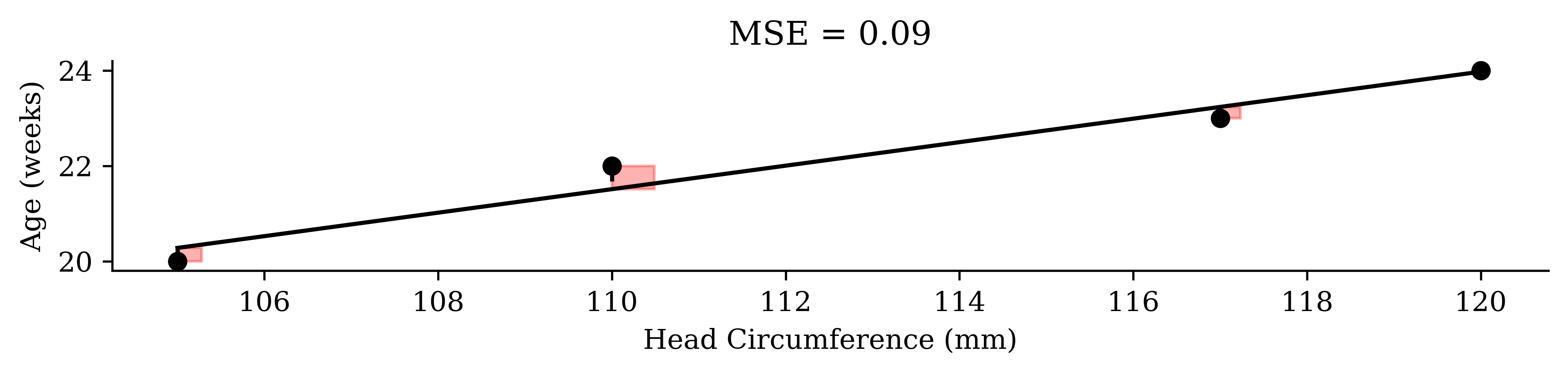

\text{MSE} = \frac{1}{n} \sum_{i=1}^n (y_i - \hat{y}_i)^2 = \frac{1}{4} \Bigl[ (-0.3)^2 + 0^2 + 0.5^2 + (-0.2)^2 \Bigr] = 0.09.

MSE in sklearn

Rather than computing the formula by hand, use mean_squared_error from sklearn.metrics.

mean_squared_error(y, model.predict(X))

0.0932971014492754

Sensitive to outliers

\text{If we instead had } \boldsymbol{y} = \begin{pmatrix} \textcolor{red}{10} & 24 & 22 & 23 \end{pmatrix}^\top.

Code

babies_outlier = pd.DataFrame({
    "circumference": [105, 120, 110, 117],
    "age": [10, 24, 22, 23],
})
X = babies_outlier[["circumference"]]
y = babies_outlier["age"]
# Predictions from the *original* model (before retraining)
predicted_age = model.predict(X)

x = babies_outlier["circumference"].to_numpy()
y = babies_outlier["age"].to_numpy()
yhat = predicted_age
error = np.abs(y - yhat)
mse = np.mean(error ** 2)

fig, ax = plt.subplots(figsize=(4, 4), dpi=300)
ax.scatter(x, y, color="black", zorder=3)
order = np.argsort(x)
ax.plot(x[order], yhat[order], color="black")
for xi, yi, yhi, ei in zip(x, y, yhat, error):
    ax.plot([xi, xi], [yi, yhi], linestyle="--", color="black")
    ax.add_patch(plt.Rectangle((xi, min(yi, yhi)), ei, ei, color="red", alpha=0.3))
ax.set_xlabel("Head Circumference (mm)")
ax.set_ylabel("Age (weeks)")
ax.set_title(f"MSE = {round(mse, 2)}")
plt.tight_layout()
plt.show()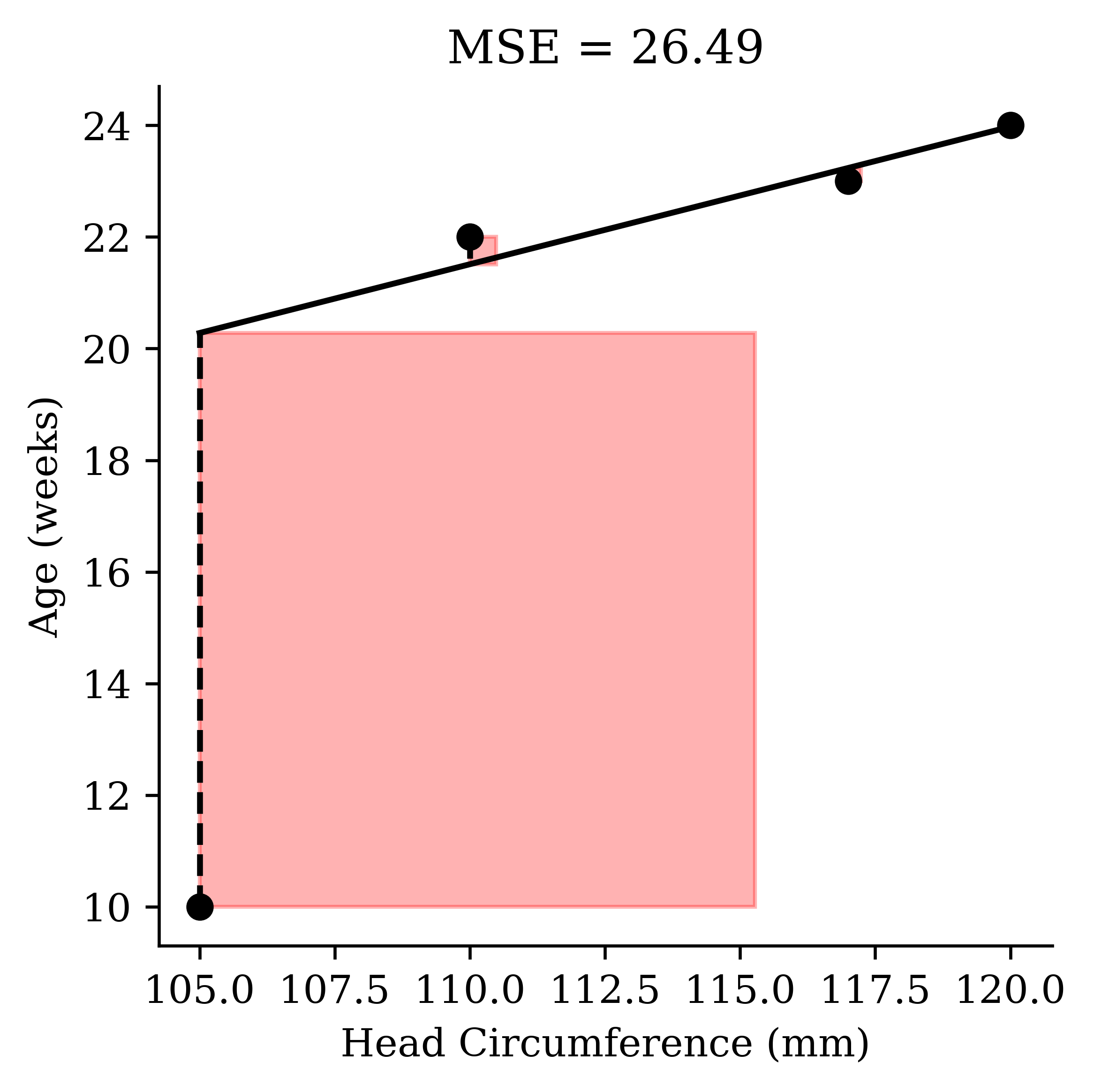

Code

new_model = LinearRegression()
new_model.fit(X, y)
predicted_age = new_model.predict(X)

x = babies_outlier["circumference"].to_numpy()
y = babies_outlier["age"].to_numpy()
yhat = predicted_age
error = np.abs(y - yhat)
mse = np.mean(error ** 2)

fig, ax = plt.subplots(figsize=(4, 4), dpi=300)
ax.scatter(x, y, color="black", zorder=3)
order = np.argsort(x)
ax.plot(x[order], yhat[order], color="black")
for xi, yi, yhi, ei in zip(x, y, yhat, error):
    ax.plot([xi, xi], [yi, yhi], linestyle="--", color="black")
    ax.add_patch(plt.Rectangle((xi, min(yi, yhi)), ei, ei, color="red", alpha=0.3))
ax.set_xlabel("Head Circumference (mm)")
ax.set_ylabel("Age (weeks)")
ax.set_title(f"MSE = {round(mse, 2)}")
plt.tight_layout()
plt.show()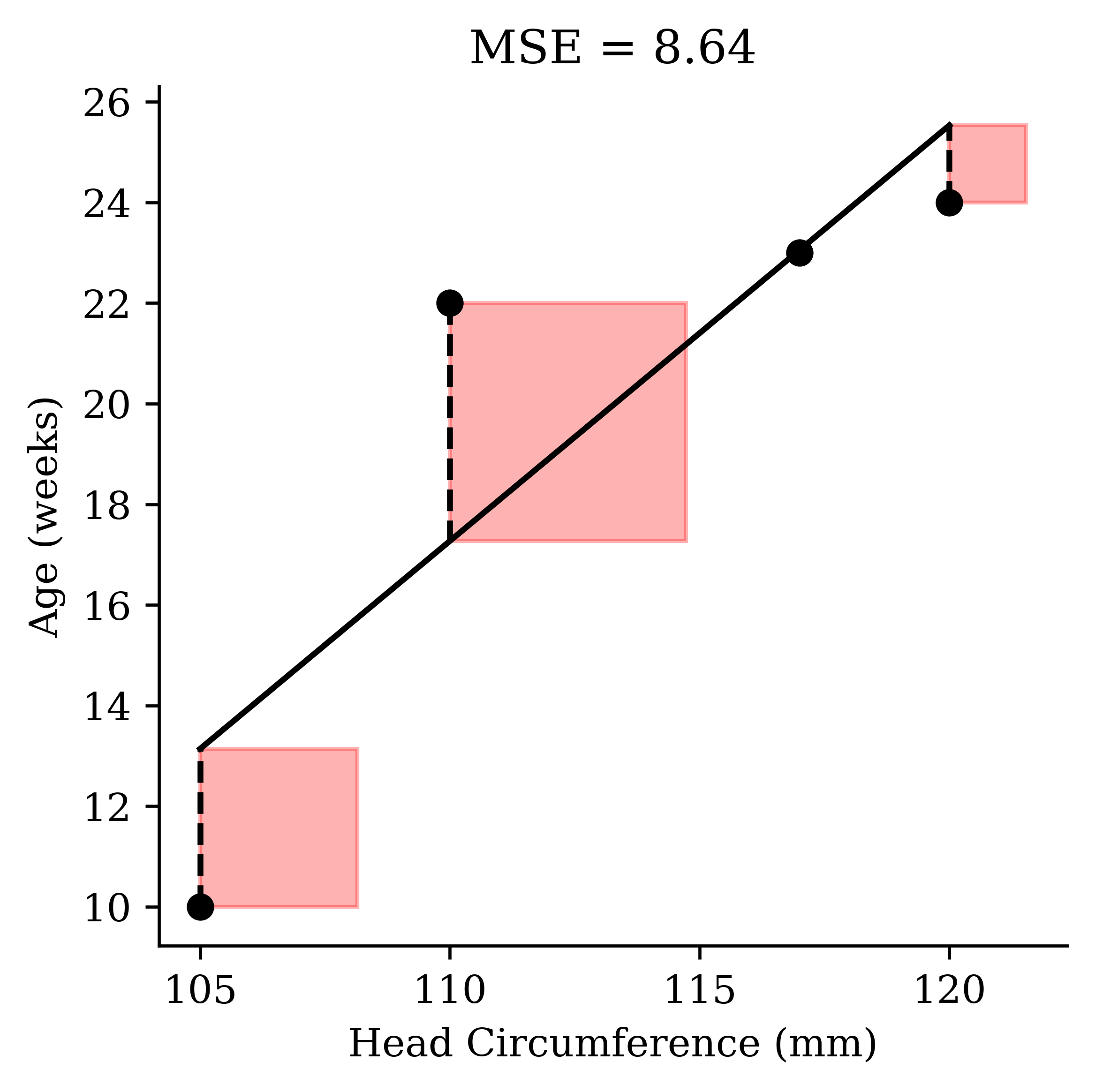

Multiple Linear Regression (MLR)

Scenario: use temperature (^\circ C) and humidity (%) to predict rainfall (mm)

\boldsymbol{X} = \begin{pmatrix} 27 & 80 \\ 32 & 70 \\ 28 & 72 \\ 22 & 86 \\ \end{pmatrix}, \quad \boldsymbol{y} = \begin{pmatrix} 6 \\ 7 \\ 6 \\ 4 \\ \end{pmatrix}, \quad \hat{\boldsymbol{y}} = \begin{pmatrix} 5.7 \\ 7.2 \\ 5.9 \\ 4.2 \\ \end{pmatrix}

\hat{y}(\boldsymbol{x}) = \beta_0 + \beta_1 x_1 + \beta_2 x_2 + \dots + \beta_p x_p = \beta_0 + \left \langle \boldsymbol{\beta}, \boldsymbol{x} \right \rangle

df = pd.DataFrame({
    "temperature": [27, 32, 28, 22],
    "humidity": [80, 70, 72, 86],
    "rainfall": [6, 7, 6, 4]
})
X = df[["temperature", "humidity"]]
y = df["rainfall"]

model = LinearRegression()
model.fit(X, y)
model.predict(X)

array([5.74, 7.2 , 5.88, 4.18])

Predict by hand

The intercept \beta_0 is in model.intercept_ and the slopes \beta_1, \dots, \beta_p are in model.coef_.

model.predict(X) gives us:

model.predict(X)

array([5.74, 7.2 , 5.88, 4.18])

We can reproduce the first entry with a for loop:

prediction = model.intercept_
for beta_j, x_0j in zip(model.coef_, X.iloc[0]):
    prediction += beta_j * x_0j
prediction

np.float64(5.739526411657559)

MLR’s design matrix

Scenario: use temperature (^\circ C) and humidity (%) to predict rainfall (mm)

\boldsymbol{X} = \begin{pmatrix} \textcolor{grey}{1} & 27 & 80 \\ \textcolor{grey}{1} & 32 & 70 \\ \textcolor{grey}{1} & 28 & 72 \\ \textcolor{grey}{1} & 22 & 86 \\ \end{pmatrix}, \quad \boldsymbol{y} = \begin{pmatrix} 6 \\ 7 \\ 6 \\ 4 \\ \end{pmatrix}, \quad \hat{\boldsymbol{y}} = \begin{pmatrix} 5.7 \\ 7.2 \\ 5.9 \\ 4.2 \\ \end{pmatrix}

\hat{y}(\boldsymbol{x}) = \beta_0 x_0 + \beta_1 x_1 + \beta_2 x_2 + \dots + \beta_p x_p = \langle \boldsymbol{\beta}, \boldsymbol{x} \rangle

print(X.to_numpy())

[[27 80]
 [32 70]
 [28 72]
 [22 86]]

X_des = np.column_stack([np.ones(len(X)), X.to_numpy()])
print(X_des)

[[ 1. 27. 80.]
 [ 1. 32. 70.]
 [ 1. 28. 72.]
 [ 1. 22. 86.]]

MLR is just matrix equations

\boldsymbol{\beta} = (\boldsymbol{X}^\top\boldsymbol{X})^{-1} \boldsymbol{X}^\top \boldsymbol{y}

model = LinearRegression()
model.fit(X, y)
print(model.intercept_, model.coef_)

-5.5100182149362436 [0.34 0.03]

beta = np.linalg.solve(
    X_des.T @ X_des, X_des.T @ y)
beta

array([-5.51,  0.34,  0.03])

\hat{\boldsymbol{y}} = \boldsymbol{X} \boldsymbol{\beta}.

model.predict(X)

array([5.74, 7.2 , 5.88, 4.18])

X_des @ beta

array([5.74, 7.2 , 5.88, 4.18])

Note, you should just use the left column. The right column’s version is for pedagogical purposes (I’ll do this kind of thing again in the upcoming slides).

MLR after normalising the inputs

Scenario: use temperature (z-score) and humidity (z-score) to predict rainfall (mm) \boldsymbol{X} = \begin{pmatrix} \textcolor{grey}{1} & -0.06 & 0.41 \\ \textcolor{grey}{1} & 1.15 & -0.95 \\ \textcolor{grey}{1} & 0.18 & -0.68 \\ \textcolor{grey}{1} & -1.28 & 1.22 \\ \end{pmatrix}, \quad \boldsymbol{y} = \begin{pmatrix} 6 \\ 7 \\ 6 \\ 4 \\ \end{pmatrix}, \quad \hat{\boldsymbol{y}} = \begin{pmatrix} 5.7 \\ 7.2 \\ 5.9 \\ 4.2 \\ \end{pmatrix}

\hat{y}(\boldsymbol{x}) = \beta_0 x_0 + \beta_1 x_1 + \beta_2 x_2 + \dots + \beta_p x_p = \langle \boldsymbol{\beta}, \boldsymbol{x} \rangle

scaler = StandardScaler()
scaler.fit(X)
X_sc = pd.DataFrame(scaler.transform(X), columns=X.columns)

model_norm = LinearRegression()
model_norm.fit(X_sc, y)
print(model_norm.intercept_, model_norm.coef_, model_norm.predict(X_sc))

5.75 [1.22 0.16] [5.74 7.2  5.88 4.18]

print(model.intercept_, model.coef_, model.predict(X))

-5.5100182149362436 [0.34 0.03] [5.74 7.2  5.88 4.18]

SLR with categorical inputs

Scenario: use property type to predict its sale price ($)

\boldsymbol{x} = \begin{pmatrix} \textcolor{red}{\text{Unit}} \\ \textcolor{green}{\text{TownHouse}} \\ \textcolor{green}{\text{TownHouse}} \\ \textcolor{blue}{\text{House}} \\ \end{pmatrix} \longrightarrow \boldsymbol{X} = \begin{pmatrix} \textcolor{grey}{1} & 1 & 0 \\ \textcolor{grey}{1} & 0 & 1 \\ \textcolor{grey}{1} & 0 & 1 \\ \textcolor{grey}{1} & 0 & 0 \\ \end{pmatrix}, \quad \boldsymbol{y} = \begin{pmatrix} 300000 \\ 500000 \\ 510000 \\ 700000 \\ \end{pmatrix}, \quad \hat{\boldsymbol{y}} = \begin{pmatrix} 300000 \\ 505000 \\ 505000 \\ 700000 \\ \end{pmatrix}

\hat{y}(x) = \beta_0 + \beta_1 \underbrace{I(x = \textcolor{red}{\text{Unit}})}_{=: x_1} + \beta_2 \underbrace{I(x = \textcolor{green}{\text{TownHouse}})}_{=: x_2} = \beta_0 + \beta_1 x_1 + \beta_2 x_2

df = pd.DataFrame({
    "type": pd.Categorical(["Unit", "TownHouse", "TownHouse", "House"]),
    "price": [300000, 500000, 510000, 700000],
})
X = pd.get_dummies(df["type"], drop_first=True, dtype=int)
y = df["price"]
model = LinearRegression()
model.fit(X, y)
print(model.intercept_, model.coef_, model.predict(X))

700000.0 [-195000. -400000.] [300000. 505000. 505000. 700000.]

Changing the base case

Scenario: use property type to predict its sale price ($)

\boldsymbol{x} = \begin{pmatrix} \textcolor{red}{\text{Unit}} \\ \textcolor{green}{\text{TownHouse}} \\ \textcolor{green}{\text{TownHouse}} \\ \textcolor{blue}{\text{House}} \\ \end{pmatrix} \longrightarrow \boldsymbol{X} = \begin{pmatrix} \textcolor{grey}{1} & 0 & 0 \\ \textcolor{grey}{1} & 1 & 0 \\ \textcolor{grey}{1} & 1 & 0 \\ \textcolor{grey}{1} & 0 & 1 \\ \end{pmatrix}, \quad \boldsymbol{y} = \begin{pmatrix} 300000 \\ 500000 \\ 510000 \\ 700000 \\ \end{pmatrix}, \quad \hat{\boldsymbol{y}} = \begin{pmatrix} 300000 \\ 505000 \\ 505000 \\ 700000 \\ \end{pmatrix}

\hat{y}(x) = \beta_0 + \beta_1 \underbrace{I(x = \textcolor{green}{\text{TownHouse}})}_{=: x_1} + \beta_2 \underbrace{I(x = \textcolor{blue}{\text{House}})}_{=: x_2} = \beta_0 + \beta_1 x_1 + \beta_2 x_2

df["type"] = df["type"].cat.reorder_categories(["Unit", "TownHouse", "House"])
X = pd.get_dummies(df["type"], drop_first=True, dtype=int)

model = LinearRegression()
model.fit(X, y)
print(model.intercept_, model.coef_, model.predict(X))

299999.99999999994 [205000. 400000.] [300000. 505000. 505000. 700000.]

Changing the target’s units

Scenario: use property type to predict its sale price ($000,000’s)

\boldsymbol{x} = \begin{pmatrix} \textcolor{red}{\text{Unit}} \\ \textcolor{green}{\text{TownHouse}} \\ \textcolor{green}{\text{TownHouse}} \\ \textcolor{blue}{\text{House}} \\ \end{pmatrix} \longrightarrow \boldsymbol{X} = \begin{pmatrix} \textcolor{grey}{1} & 0 & 0 \\ \textcolor{grey}{1} & 1 & 0 \\ \textcolor{grey}{1} & 1 & 0 \\ \textcolor{grey}{1} & 0 & 1 \\ \end{pmatrix}, \quad \boldsymbol{y} = \begin{pmatrix} 0.3 \\ 0.5 \\ 0.51 \\ 0.7 \\ \end{pmatrix}, \quad \hat{\boldsymbol{y}} = \begin{pmatrix} 0.3 \\ 0.505 \\ 0.505 \\ 0.7 \\ \end{pmatrix}

df["price"] /= 1e6
y = df["price"]

model = LinearRegression()
model.fit(X, y)
print(model.intercept_, model.coef_, model.predict(X))

0.2999999999999999 [0.21 0.4 ] [0.3  0.51 0.51 0.7 ]

Dates as categorical inputs

Imagine you had dataset with 157,209 rows and one covariate column was ‘date of birth’. There were 27,485 unique values for the date of birth column. You make a linear regression with the date of birth as an input, and treat it as a categorical variable.

Pandas/sklearn would make a design matrix of size 157,209 \times 27,485. This has 4,320,889,365 numbers in it. Each number is stored as 8 bytes, so the matrix is roughly 34,000,000,000 \text{ bytes} = 34,000,000 \text{ KB} = 34,000 \text{ MB} = 34 \text{ GB}.

Question: How do we avoid this situation of crashing our computer with an ‘out of memory’ error?

Solution: Don’t train on the date of birth — at least, not as a categorical variable. Turn it into a numerical variable, e.g. age. If the date column were not ‘date of birth’, maybe calculate the number of days since some reference date, or split into day, month, year columns.

Generalised Linear Models Recap

MLR with categorical targets

Scenario: use tumour radius (mm) and ages (years) to predict benign or malignant \boldsymbol{X} = \begin{pmatrix} \textcolor{grey}{1} & 14.8 & 48 \\ \textcolor{grey}{1} & 16.4 & 49 \\ \textcolor{grey}{1} & 15.5 & 47 \\ \textcolor{grey}{1} & 14.2 & 46 \\ \end{pmatrix}, \quad \boldsymbol{y} = \begin{pmatrix} \text{Benign} \\ \text{Malignant} \\ \text{Benign} \\ \text{Malignant} \\ \end{pmatrix}, \quad \hat{\boldsymbol{y}} = \begin{pmatrix} ? \\ ? \\ ? \\ ? \\ \end{pmatrix}

Step 1: Make a linear prediction \beta_0 + \beta_1 x_1 + \dots + \beta_p x_p , \quad \text{a.k.a.} \quad \langle \boldsymbol{\beta}, \boldsymbol{x} \rangle.

Step 2: Shove it through some function to make it a probability \sigma(\langle \boldsymbol{\beta}, \boldsymbol{x} \rangle) Interpret that as being the probability of the positive class.

Step 3: Make a decision based on that probability. E.g., if the probability is greater than 0.5, predict the positive class.

Binomial regression with sklearn

Scenario: use tumour radius (mm) and ages (years) to predict benign or malignant \boldsymbol{y} = \begin{pmatrix} \text{Benign} \\ \textbf{\text{Malignant}} \\ \text{Benign} \\ \textbf{\text{Malignant}} \\ \end{pmatrix}, \quad \sigma( \boldsymbol{X} \boldsymbol{\beta} ) = \begin{pmatrix} 39\% \\ 55\% \\ 59\% \\ 48\% \\ \end{pmatrix} , \quad \hat{\boldsymbol{y}} = \begin{pmatrix} \text{Benign} \\ \text{Malignant} \\ \text{Malignant} \\ \text{Benign} \\ \end{pmatrix}

Load the data, fit a GLM, make predictions:

patients = pd.DataFrame({
    "radius": [14.8, 16.4, 15.5, 14.2],
    "age": [48, 49, 47, 46],
    "tumour": ["Benign", "Malignant", "Benign", "Malignant"],
})
X = patients[["radius", "age"]]
y = patients["tumour"]

model = LogisticRegression(C=np.inf)
model.fit(X, y)
model.predict(X)

array(['Benign', 'Malignant', 'Malignant', 'Benign'], dtype=object)

Binomial regression I

Scenario: use tumour radius (mm) and ages (years) to predict benign or malignant \boldsymbol{X} = \begin{pmatrix} \textcolor{grey}{1} & 14.8 & 48 \\ \textcolor{grey}{1} & 16.4 & 49 \\ \textcolor{grey}{1} & 15.5 & 47 \\ \textcolor{grey}{1} & 14.2 & 46 \\ \end{pmatrix}, \quad \boldsymbol{y} = \begin{pmatrix} \text{Benign} \\ \textbf{\text{Malignant}} \\ \text{Benign} \\ \textbf{\text{Malignant}} \\ \end{pmatrix}, \quad \boldsymbol{X} \boldsymbol{\beta} = \begin{pmatrix} -0.46 \\ 0.18 \\ 0.37 \\ -0.09 \\ \end{pmatrix}

model = LogisticRegression(C=np.inf)
model.fit(X, y);

Step 1: Make a linear prediction

linear = model.decision_function(X)
linear

array([-0.46,  0.18,  0.37, -0.09])

X_des = np.column_stack([np.ones(len(X)), X.to_numpy()])
beta = np.concatenate([model.intercept_, model.coef_.flatten()])
X_des @ beta

array([-0.46,  0.18,  0.37, -0.09])

Logistic regression and probit regression

Code

def sigmoid(x):
    return 1 / (1 + np.exp(-x))

xs = np.arange(-6, 6, 0.1)
ys = sigmoid(xs)

fig, ax = plt.subplots(figsize=(3, 3))
ax.plot(xs, ys, linewidth=1.5)
ax.set_xlabel("x")
ax.set_ylabel("y")
ax.set_title("Sigmoid function")
plt.show()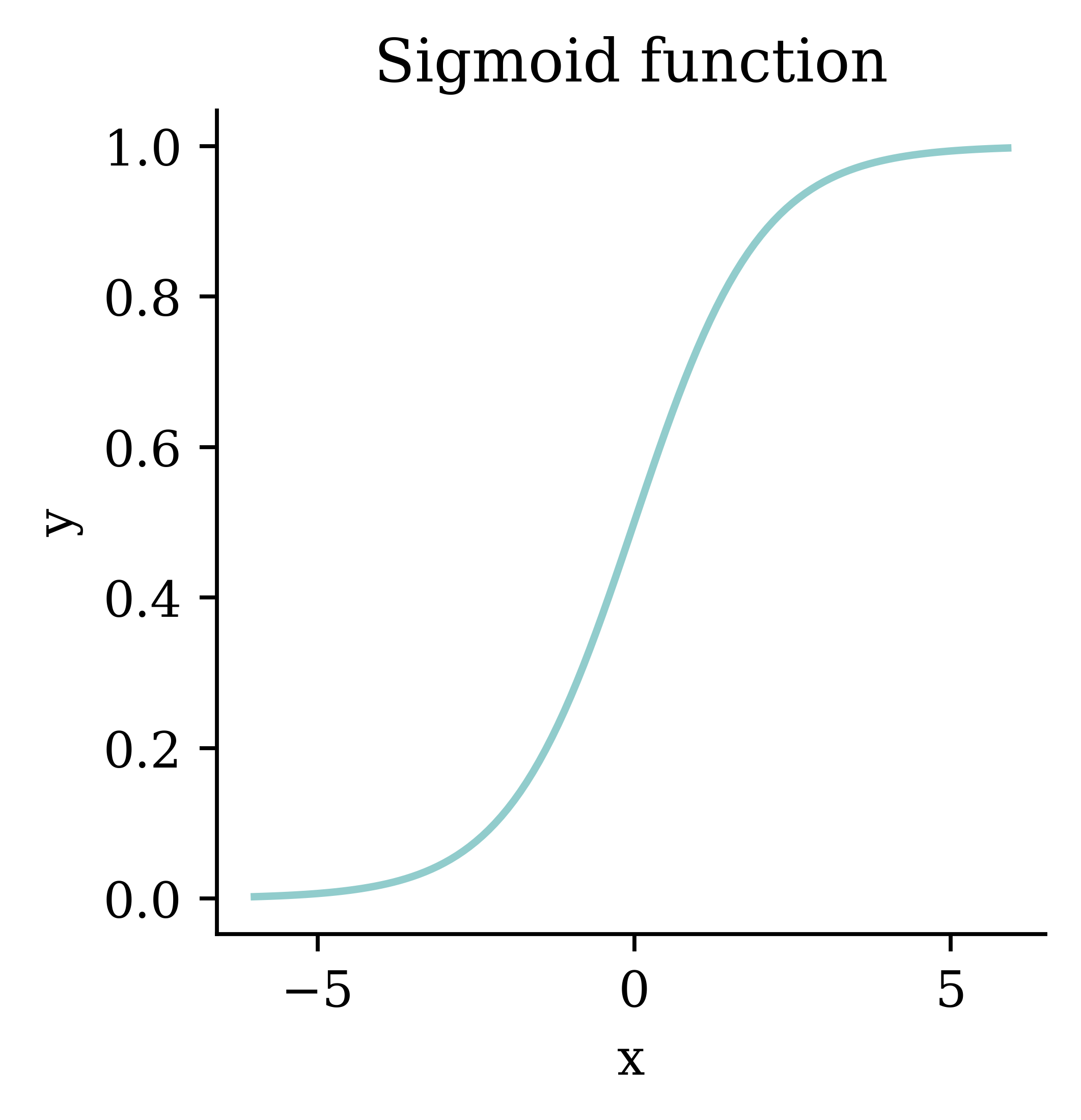

This give you logistic regression.

Code

from scipy.stats import norm

xs = np.arange(-6, 6, 0.1)
ys = norm.cdf(xs)

fig, ax = plt.subplots(figsize=(3, 3))
ax.plot(xs, ys, linewidth=1.5)
ax.set_xlabel("x")
ax.set_ylabel("y")
ax.set_title("Normal CDF function")
plt.show()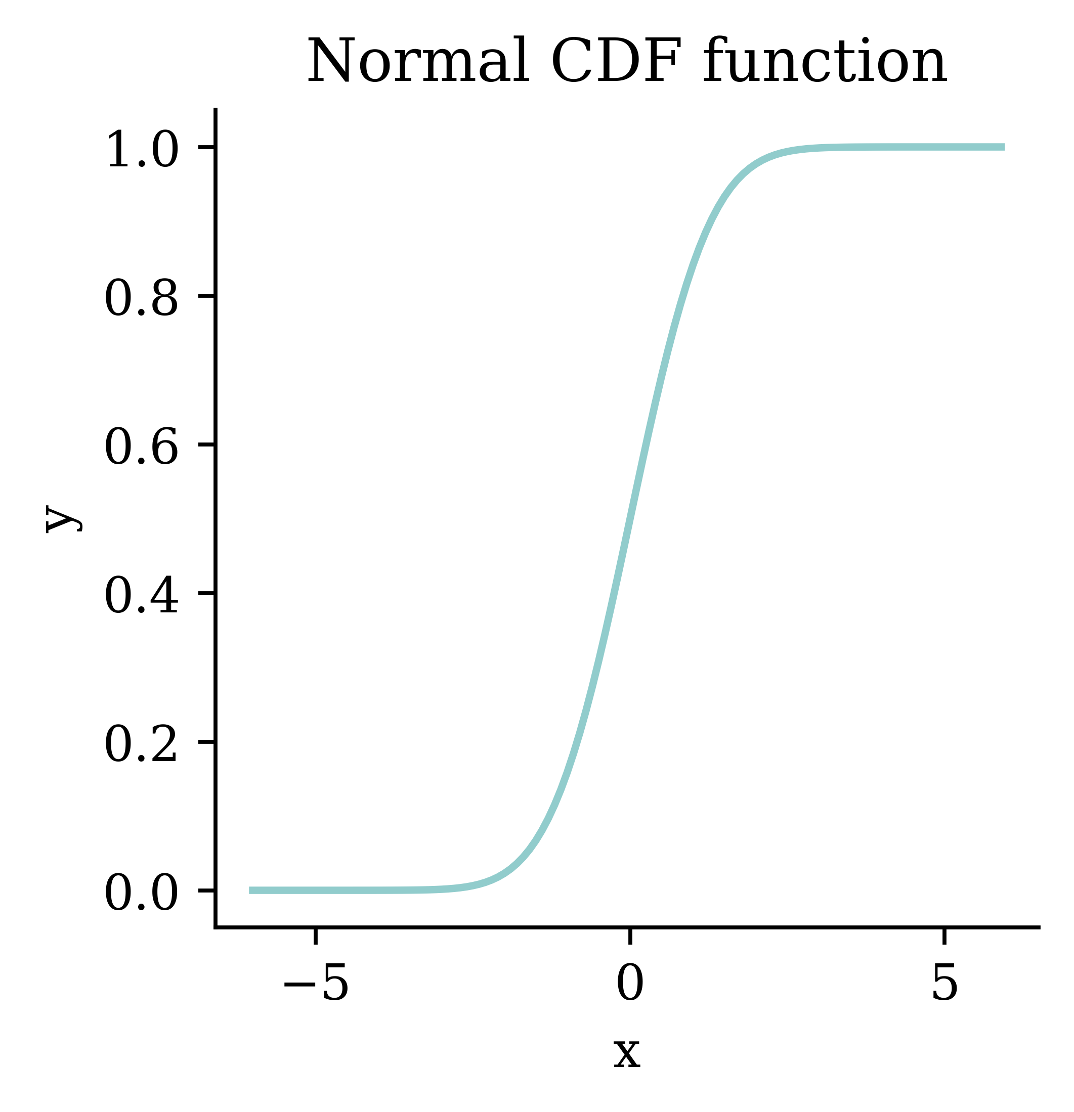

This gives you probit regression.

Logistic Regression

Scenario: use tumour radius (mm) and ages (years) to predict benign or malignant \boldsymbol{y} = \begin{pmatrix} \text{Benign} \\ \textbf{\text{Malignant}} \\ \text{Benign} \\ \textbf{\text{Malignant}} \\ \end{pmatrix}, \quad \boldsymbol{X} \boldsymbol{\beta} = \begin{pmatrix} -0.46 \\ 0.18 \\ 0.37 \\ -0.09 \\ \end{pmatrix}, \quad \sigma( \boldsymbol{X} \boldsymbol{\beta} ) = \begin{pmatrix} 39\% \\ 55\% \\ 59\% \\ 48\% \\ \end{pmatrix}

model = LogisticRegression(C=np.inf)
model.fit(X, y)
linear = model.decision_function(X)

Step 2: Shove it through some function to make it a probability

sigmoid(linear)

array([0.39, 0.55, 0.59, 0.48])

model.predict_proba(X)[:, 1] # Probability of the positive class (Malignant)

array([0.39, 0.55, 0.59, 0.48])

Predicting categories

model = LogisticRegression(C=np.inf)
model.fit(X, y);

predict_probs = model.predict_proba(X)[:, 1]
cutoff = 0.5
predicted_tumours = np.where(predict_probs > cutoff, "Malignant", "Benign")
print(predicted_tumours)

['Benign' 'Malignant' 'Malignant' 'Benign']

Assessing accuracy in classification problems

Scenario: use tumour radius (mm) and ages (years) to predict benign or malignant \boldsymbol{y} = \begin{pmatrix} \textcolor{Green}{\text{Benign}} \\ \textcolor{Green}{\text{Malignant}} \\ \textcolor{Red}{\text{Benign}} \\ \textcolor{Red}{\text{Malignant}} \\ \end{pmatrix}, \quad \hat{\boldsymbol{y}} = \begin{pmatrix} \textcolor{Green}{\text{Benign}} \\ \textcolor{Green}{\text{Malignant}} \\ \textcolor{Red}{\text{Malignant}} \\ \textcolor{Red}{\text{Benign}} \\ \end{pmatrix}

Accuracy: \frac{1}{n}\sum_{i=1}^n I(y_i = \hat{y}_i)

Error rate: \frac{1}{n}\sum_{i=1}^n I(y_i \neq \hat{y}_i)

Note

The word “accuracy” is used often used loosely when discussing models, particularly regression models. In the context of classification it has this specific meaning.

Decision Tree

model = DecisionTreeClassifier(min_samples_split=2)
model.fit(X, y)

plot_tree(model, feature_names=list(X.columns), class_names=model.classes_, filled=True);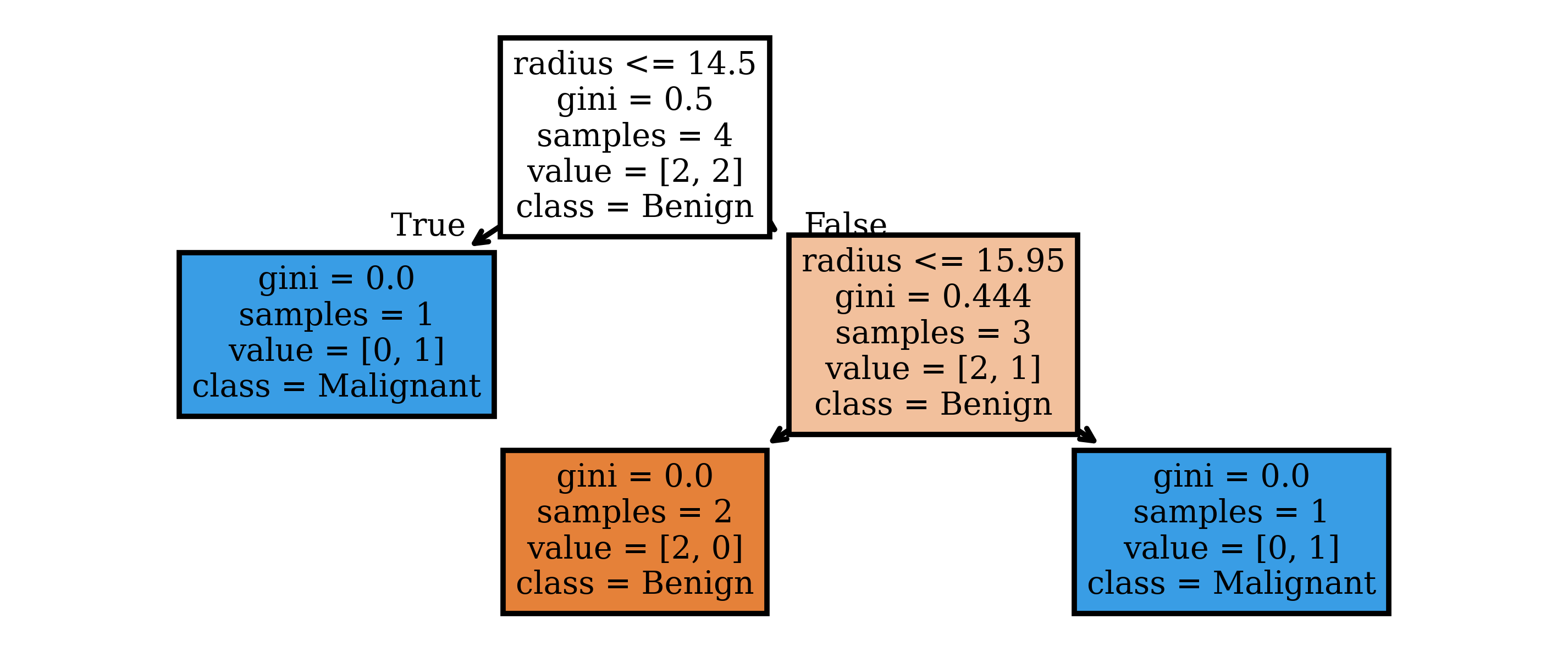

Poisson regression

Scenario: use population density to predict the daily count of gun violence incidents

\boldsymbol{X} = \begin{pmatrix} \textcolor{grey}{1} & 10 \\ \textcolor{grey}{1} & 15 \\ \textcolor{grey}{1} & 12 \\ \textcolor{grey}{1} & 18 \\ \end{pmatrix}, \quad \boldsymbol{y} = \begin{pmatrix} 155 \\ 208 \\ 116 \\ 301 \\ \end{pmatrix}, \quad \hat{\boldsymbol{y}} = \begin{pmatrix} ? \\ ? \\ ? \\ ? \\ \end{pmatrix}

Step 1: Make a linear prediction \beta_0 + \beta_1 x_1 + \dots + \beta_p x_p , \quad \text{a.k.a.} \quad \langle \boldsymbol{\beta}, \boldsymbol{x} \rangle.

Step 2: Shove it through some function to make it positive \exp(\langle \boldsymbol{\beta}, \boldsymbol{x} \rangle) Interpret that as being the expected count.

Predict the mean of a Poisson distribution I

Scenario: use population density to predict the daily count of gun violence incidents

\boldsymbol{X} = \begin{pmatrix} \textcolor{grey}{1} & 10 \\ \textcolor{grey}{1} & 15 \\ \textcolor{grey}{1} & 12 \\ \textcolor{grey}{1} & 18 \\ \end{pmatrix}, \quad \boldsymbol{y} = \begin{pmatrix} 155 \\ 208 \\ 116 \\ 301 \\ \end{pmatrix}, \quad \boldsymbol{X} \boldsymbol{\beta} = \begin{pmatrix} 4.82 \\ 5.35 \\ 5.03 \\ 5.67 \\ \end{pmatrix}, \quad \hat{\boldsymbol{\mu}} = \begin{pmatrix} 125.1 \\ 211.3 \\ 154.3 \\ 289.4 \\ \end{pmatrix}

Load the data, fit the model, and make a prediction.

guns = pd.DataFrame({
    "density": [10, 15, 12, 18],
    "incidents": [155, 208, 116, 301],
})
X = guns[["density"]]
y = guns["incidents"]

model = PoissonRegressor(alpha=0)
model.fit(X, y)

print(model.predict(X))

[125.08 211.28 154.26 289.38]

Predict the mean of a Poisson distribution II

Scenario: use population density to predict the daily count of gun violence incidents

\boldsymbol{X} = \begin{pmatrix} \textcolor{grey}{1} & 10 \\ \textcolor{grey}{1} & 15 \\ \textcolor{grey}{1} & 12 \\ \textcolor{grey}{1} & 18 \\ \end{pmatrix}, \quad \boldsymbol{y} = \begin{pmatrix} 155 \\ 208 \\ 116 \\ 301 \\ \end{pmatrix}, \quad \boldsymbol{X} \boldsymbol{\beta} = \begin{pmatrix} 4.82 \\ 5.35 \\ 5.03 \\ 5.67 \\ \end{pmatrix}, \quad \hat{\boldsymbol{\mu}} = \begin{pmatrix} 125.1 \\ 211.3 \\ 154.3 \\ 289.4 \\ \end{pmatrix}

These are the linear coefficients:

print(model.intercept_, model.coef_)

3.7803728824634275 [0.1]

Step 1: Make linear predictions

X_des = np.column_stack([np.ones(len(X)), X.to_numpy()])
beta = np.concatenate([[model.intercept_], model.coef_])
linear = X_des @ beta
print(linear)

[4.83 5.35 5.04 5.67]

Predict the mean of a Poisson distribution III

Scenario: use population density to predict the daily count of gun violence incidents

\boldsymbol{X} = \begin{pmatrix} \textcolor{grey}{1} & 10 \\ \textcolor{grey}{1} & 15 \\ \textcolor{grey}{1} & 12 \\ \textcolor{grey}{1} & 18 \\ \end{pmatrix}, \quad \boldsymbol{y} = \begin{pmatrix} 155 \\ 208 \\ 116 \\ 301 \\ \end{pmatrix}, \quad \boldsymbol{X} \boldsymbol{\beta} = \begin{pmatrix} 4.82 \\ 5.35 \\ 5.03 \\ 5.67 \\ \end{pmatrix}, \quad \hat{\boldsymbol{\mu}} = \begin{pmatrix} 125.1 \\ 211.3 \\ 154.3 \\ 289.4 \\ \end{pmatrix}

Step 2: Exponentiate it

linear = X_des @ beta
print(np.exp(linear))

[125.08 211.28 154.26 289.38]

model.predict(X)

array([125.08, 211.28, 154.26, 289.38])

California House Price Prediction (Setup)

Data science always starts with the data!

The target variable is the median house value for California districts, expressed in $100,000’s. This dataset was derived from the 1990 U.S. census, using one row per census block group. A block group is the smallest geographical unit for which the U.S. Census Bureau publishes sample data (a block group typically has a population of 600 to 3,000 people).

Columns

MedInc median income in block group
HouseAge median house age in block group
AveRooms average number of rooms per household
AveBedrms average # of bedrooms per household
Population block group population
AveOccup average number of household members
Latitude block group latitude
Longitude block group longitude
MedHouseVal median house value (target)

Import the data

1features, target = fetch_california_housing(as_frame=True, return_X_y=True)
features

1: Assigns features and target from the dataset to two variables ‘features’ and ‘target’ and returns two separate data frames. The command return_X_y=True ensures that there will be two separate data frames, one for the features and the other for the target

	MedInc	HouseAge	AveRooms	AveBedrms	Population	AveOccup	Latitude	Longitude
0	8.3252	41.0	6.984127	1.023810	322.0	2.555556	37.88	-122.23
1	8.3014	21.0	6.238137	0.971880	2401.0	2.109842	37.86	-122.22
2	7.2574	52.0	8.288136	1.073446	496.0	2.802260	37.85	-122.24
...	...	...	...	...	...	...	...	...
20637	1.7000	17.0	5.205543	1.120092	1007.0	2.325635	39.43	-121.22
20638	1.8672	18.0	5.329513	1.171920	741.0	2.123209	39.43	-121.32
20639	2.3886	16.0	5.254717	1.162264	1387.0	2.616981	39.37	-121.24

20640 rows × 8 columns

What is the target?

target

0        4.526
1        3.585
2        3.521
         ...  
20637    0.923
20638    0.847
20639    0.894
Name: MedHouseVal, Length: 20640, dtype: float64

Why predict this? Let’s pretend we are these guys.

Apply the three-way split to California housing

The same train_test_split pattern, now applied to the loaded data:

X_main, X_test, y_main, y_test = train_test_split(features, target, test_size=0.2, random_state=1)
X_train, X_val, y_train, y_val = train_test_split(X_main, y_main, test_size=0.25, random_state=1)
print(X_train.shape, X_val.shape, X_test.shape)

(12384, 8) (4128, 8) (4128, 8)

A 60:20:20 three-way split: 20\% for the held-out test set, then 25\% of the remaining 80\% (i.e. 20\% overall) for the validation set, leaving 60\% for training. The same random_state would let a teammate reproduce the split exactly.

The training set

X_train

	MedInc	HouseAge	AveRooms	AveBedrms	Population	AveOccup	Latitude	Longitude
9107	4.1573	19.0	6.162630	1.048443	1677.0	2.901384	34.63	-118.18
13999	0.4999	10.0	6.740000	2.040000	108.0	2.160000	34.69	-116.90
5610	2.0458	27.0	3.619048	1.062771	1723.0	3.729437	33.78	-118.26
...	...	...	...	...	...	...	...	...
8539	4.0727	18.0	3.957845	1.079625	2276.0	2.665105	33.90	-118.36
2155	2.3190	41.0	5.366265	1.113253	1129.0	2.720482	36.78	-119.79
13351	5.5632	9.0	7.241087	0.996604	2280.0	3.870968	34.02	-117.62

12384 rows × 8 columns

Location

Python’s matplotlib package \approx R’s basic plots.

plt.scatter(features["Longitude"], features["Latitude"])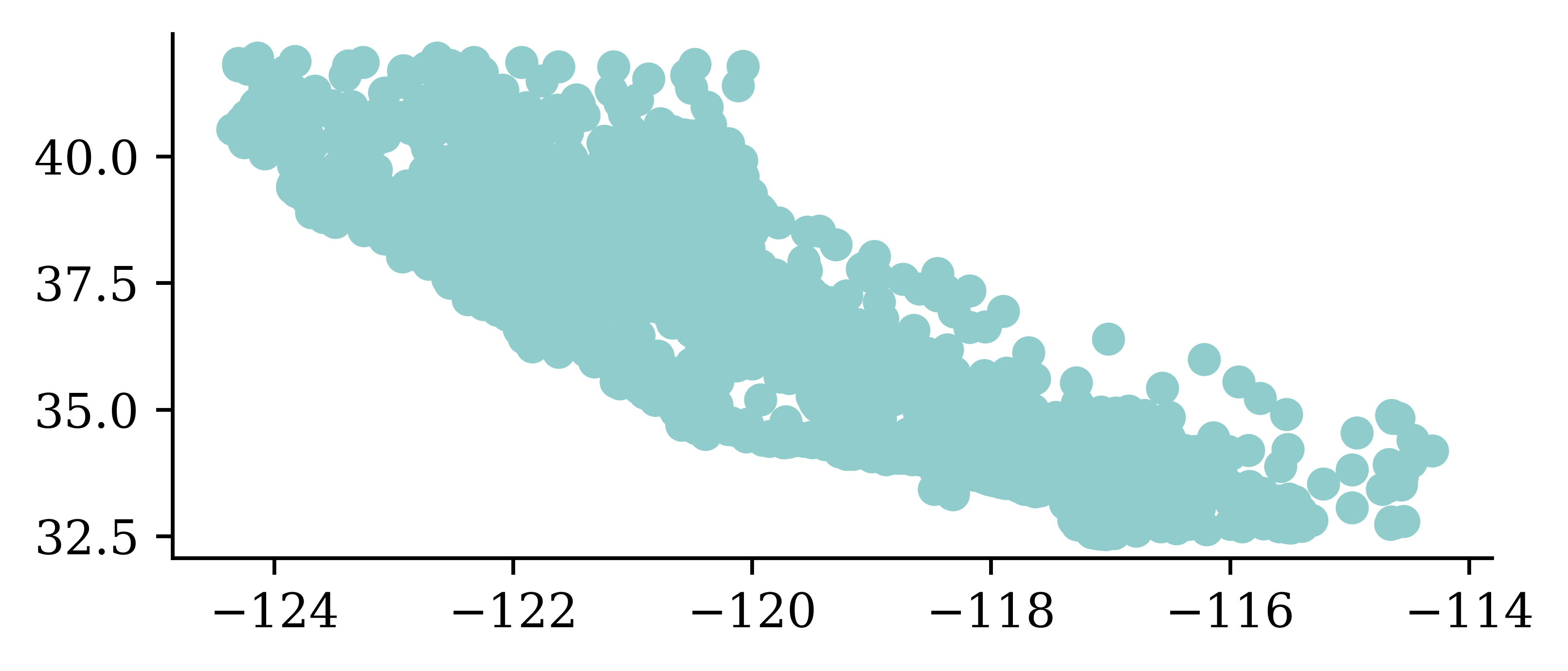

Note

There’s no analysis in this EDA.

Location EDA

plt.scatter(features["Longitude"], features["Latitude"], c=target, cmap="coolwarm")
plt.colorbar()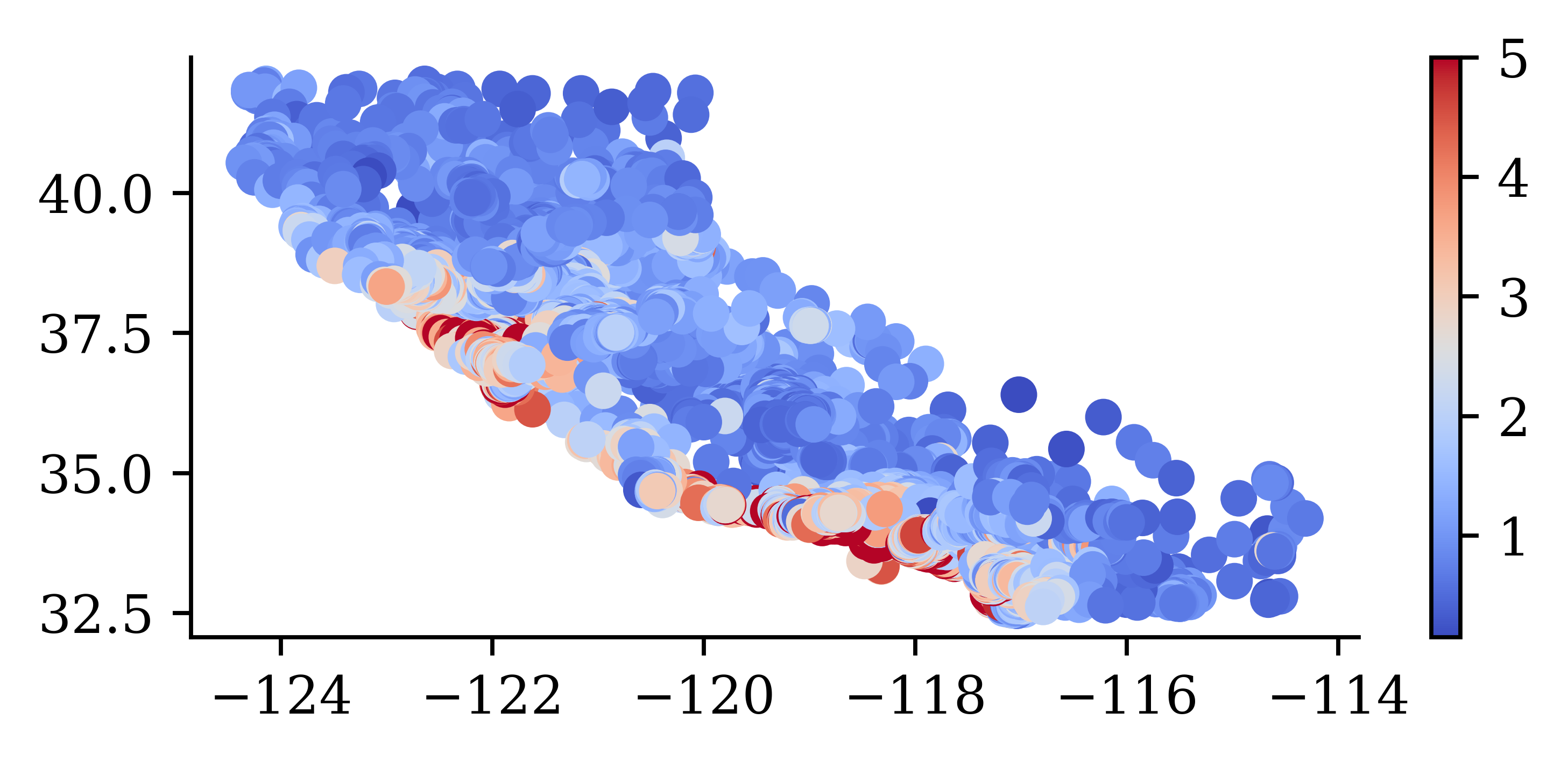

“We observe that the median house prices are higher closer to the coastline.”

Pandas can make plots directly

both = pd.concat([features, target], axis=1)
both.plot(kind="scatter", x="Longitude", y="Latitude", c="MedHouseVal", cmap="coolwarm")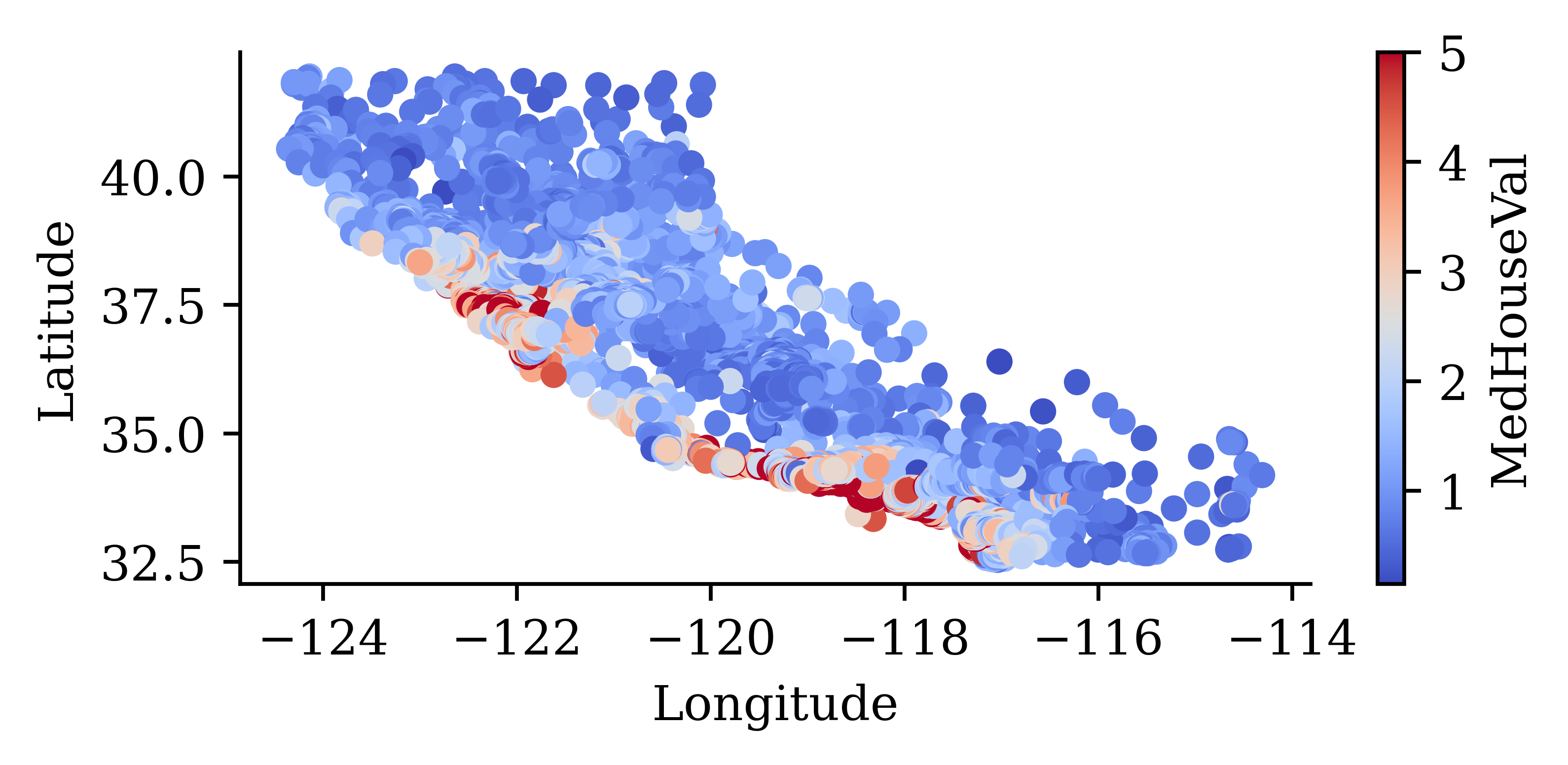

Features

print(list(features.columns))

['MedInc', 'HouseAge', 'AveRooms', 'AveBedrms', 'Population', 'AveOccup', 'Latitude', 'Longitude']

How many?

num_features = len(features.columns)
num_features

num_features = features.shape[1]
features.shape

(20640, 8)

California House Price Prediction (Regression)

Linear Regression

\hat{y}_i = w_0 + \sum_{j=1}^p w_j x_{ij} .

1lr = LinearRegression()
2lr.fit(X_train, y_train);

1: Defines the object lr which represents the linear regression function.
2: Fits a linear regression model using the training data. lr.fit computes the coefficients of the regression model.

The w_0 is in lr.intercept_ and the others are in

print(lr.coef_)

[ 4.34e-01  9.88e-03 -9.40e-02  5.86e-01 -1.58e-06 -3.60e-03 -4.26e-01
 -4.42e-01]

Make some predictions

X_train.head(3)

	MedInc	HouseAge	AveRooms	AveBedrms	Population	AveOccup	Latitude	Longitude
9107	4.1573	19.0	6.162630	1.048443	1677.0	2.901384	34.63	-118.18
13999	0.4999	10.0	6.740000	2.040000	108.0	2.160000	34.69	-116.90
5610	2.0458	27.0	3.619048	1.062771	1723.0	3.729437	33.78	-118.26

X_train.head(3) returns the first three rows of the dataset X_train.

y_pred = lr.predict(X_train.head(3))
y_pred

array([1.82, 0.08, 1.62])

lr.predict(X_train.head(3)) returns the predictions for the first three rows of the dataset X_train.

Plot the predictions

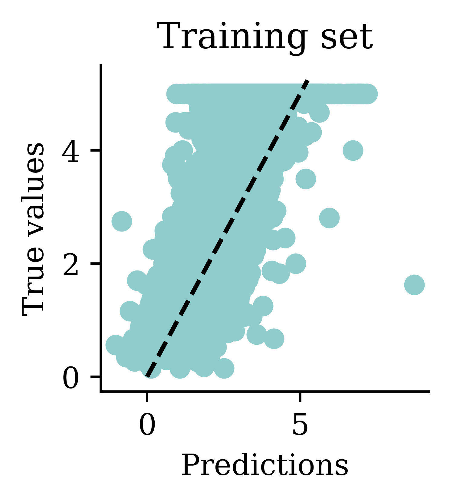
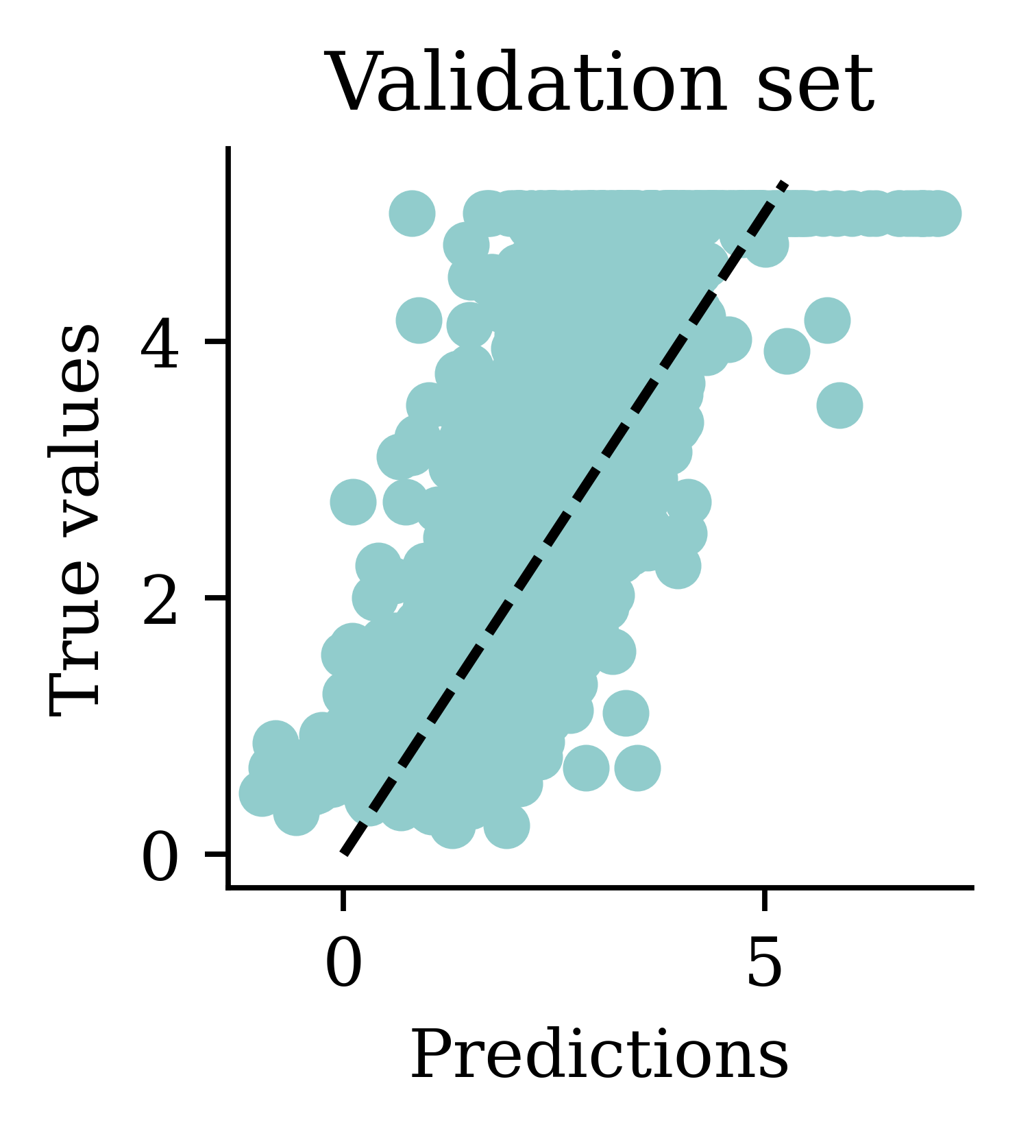
We can see dispersion around the fitted line.

Track MSE for model comparison

We’ll add ANN results to these dictionaries later.

mse_lr_train = mean_squared_error(y_train, lr.predict(X_train))
mse_lr_val = mean_squared_error(y_val, lr.predict(X_val))

mse_train = {"Linear Regression": mse_lr_train}
mse_val = {"Linear Regression": mse_lr_val}

Tip

Think about the units of the mean squared error. Is there a variation which is more interpretable?

To be continued…

We’ll revisit this California housing problem in the AI and Deep Learning lecture, where we extend mse_train and mse_val with neural network results and compare them against this linear regression baseline.

References

Package Versions

from watermark import watermark
print(watermark(python=True, packages="matplotlib,numpy,pandas,seaborn,scikit-learn,scipy"))

Python implementation: CPython
Python version       : 3.14.3
IPython version      : 9.13.0

matplotlib  : 3.10.9
numpy       : 2.4.4
pandas      : 3.0.2
seaborn     : 0.13.2
scikit-learn: 1.8.0
scipy       : 1.17.1

Glossary

base case (in dummy encoding)
categorical input / dummy encoding
design matrix
exploratory data analysis (EDA)
features, target
generalised linear model (GLM)
linear regression
link function
logistic regression
matplotlib

mean squared error
numpy
pandas DataFrame
Poisson regression
probit regression
scikit-learn (fit / predict / score)
sigmoid function
standardisation (z-score)
train_test_split
training / validation / test split

References

James, G., Witten, D., Hastie, T., & Tibshirani, R. (2021). An Introduction to Statistical Learning: with Applications in R. Springer.