Lab: Time Series & Recurrent Neural Networks
ACTL3143 & ACTL5111 Deep Learning for Actuaries
Part 1: Time series as ordered data
Exercise 1: Tabular data versus time-series data
In a standard supervised-learning problem, we often write observations as
\{(x_i, y_i)\}_{i=1}^n.
In a time-series problem, observations arrive in order:
\{(x_t, y_t)\}_{t=1}^T.
- What is the difference between the index i and the time index t?
- Why does the order of observations matter in a time-series problem?
- Why might the independence assumption be less reasonable for time-series data?
Exercise 2: Examples of sequence problems
For each of the following applications, identify the input sequence and the prediction target.
- Forecasting future claim payments.
- Forecasting mortality rates over calendar years.
- Forecasting daily stock returns.
- Forecasting tomorrow’s temperature.
- Predicting the next word in a sentence.
For each example, also decide whether the sequence is naturally indexed by time or by position in a sequence.
Exercise 3: Prediction target and information available at time t
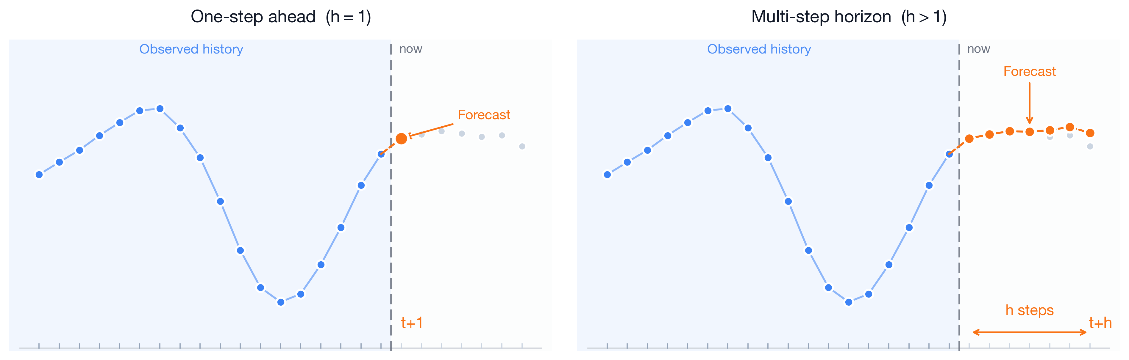
Suppose that at each time point t, we observe predictors x_t and a response y_t.
A common forecasting problem is to predict y_{t+1} using information available up to time t:
(x_1, y_1), (x_2, y_2), \ldots, (x_t, y_t) \quad \longrightarrow \quad y_{t+1}.
- What information is available when predicting y_{t+1}?
- If x_{t+1} is only observed at time t+1, should it be used to predict y_{t+1} at time t?
- In a real forecasting problem, why is it important to define the prediction time clearly?
Exercise 4: Trend, seasonality and noise
Consider a daily temperature series.
- What is meant by trend, seasonality and noise?
- Which of these components would you expect to be important for weather data?
- Which of these components would you expect to be important for daily stock returns?
- If we use only the previous 7 days of temperature to predict tomorrow’s temperature, can the model easily learn annual seasonality?
- What extra information could we give to an RNN to help it learn seasonal patterns?
- Why might sine and cosine transformations of the day of year be useful seasonal features?
Part 2: Classical time-series models
Before using RNNs, it is useful to understand classical time-series models and simple baselines.
An autoregressive model uses previous values of the series to predict the next value. For example,
y_t = \alpha + \phi_1 y_{t-1} + \epsilon_t.
ARIMA models extend this idea by combining autoregression, differencing, and moving-average errors.
Answer the following questions.
- In the autoregressive model above, what does y_{t-1} represent?
- What does the coefficient \phi_1 measure?
- Why might differencing be useful when the series has a trend?
- What is a persistence forecast?
- What is a seasonal naive forecast?
- Why should an RNN be compared against simple baselines such as persistence or seasonal naive forecasts?
- Why might ARIMA be a strong method for a single short time series?
- Why might RNNs be more attractive when we have many related sequences or many predictors?
Part 3: Simple recurrent neural networks
Exercise 5: RNN intuition
A SimpleRNN processes a sequence one step at a time.
At time t, the hidden state is updated using the current input and the previous hidden state:
h_t = f(W_x x_t + W_h h_{t-1} + b).
- What is x_t, h_{t-1} and h_t?
- Why does the hidden state act like a memory?
- What role does the activation function f play?
Exercise 6: Reusing weights across time
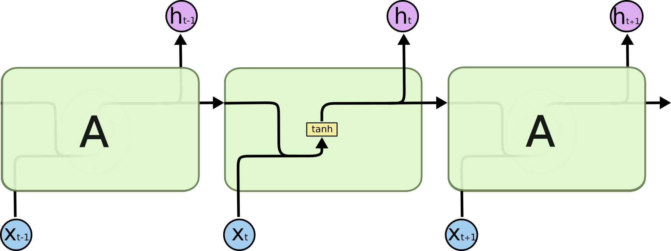
In an RNN, the same weight matrices are used at every time step.
- Why is this different from using a separate dense layer for each time step?
- Why does weight sharing make sense for sequence data?
- How does weight sharing reduce the number of parameters?
- What would happen to the number of parameters if we used separate weights for every time step?
Exercise 7: Manual RNN calculation
Consider a very small RNN with scalar inputs and scalar hidden states:
h_t = \tanh(w_x x_t + w_h h_{t-1} + b).
Let
w_x = 0.5,\quad w_h = 0.2,\quad b = 0,\quad h_0 = 0.
For the input sequence
x_1 = 2,\quad x_2 = 1,
calculate:
- h_1;
- h_2.
You may leave your answers in terms of \tanh(\cdot).
Exercise 8: Interpreting RNN input shape
An RNN input array has dimension
(1000, 10, 3).
Interpret this dimension vector.
- What does the first dimension, 1000, represent?
- What does the second dimension, 10, represent?
- What does the third dimension, 3, represent?
- How many values are contained in one sequence?
- If this is daily weather data, give an example of what the 3 features at each time step could be.
- Why does an RNN require this three-dimensional structure instead of a two-dimensional matrix?
Exercise 9: RNNs for text sequences
RNNs can also be used for natural language processing because text is ordered sequence data.
Consider the sentence:
\text{``The policyholder reported a car accident.''}
- What are the sequence elements in this sentence?
- Why does word order matter in text?
- How could the words be converted into numerical inputs for an RNN?
- If we use an RNN to classify accident reports into severity classes, what is the input sequence and what is the prediction target?
Exercise 10: Many-to-one and many-to-many problems
For each task below, decide whether it is many-to-one or many-to-many.
- Use the last 20 days of weather variables to predict tomorrow’s weather class.
- Use a sentence to predict whether a review is positive or negative.
- Translate an English sentence into French.
- Predict the next value at every time point in a sequence.
- Use a patient’s history to predict whether they will be hospitalised next month.
Part 4: Limitations of SimpleRNN
Exercise 11: Long-term dependence
SimpleRNNs can struggle with long sequences.
- What does long-term dependence mean?
- Why might yesterday’s temperature be more useful than the temperature 300 days ago?
- Give an example where information from much earlier in the sequence could still matter.
- Why might SimpleRNNs have difficulty learning this?
Exercise 12: Vanishing gradients
When training an RNN, gradients are propagated backward through time.
- What does “backward through time” mean?
- What is the vanishing-gradient problem?
- Why does this make it difficult to learn long-term dependencies?
- Why is this problem less severe for short sequences?
Part 5: LSTM and GRU
Exercise 13: Motivation for LSTM
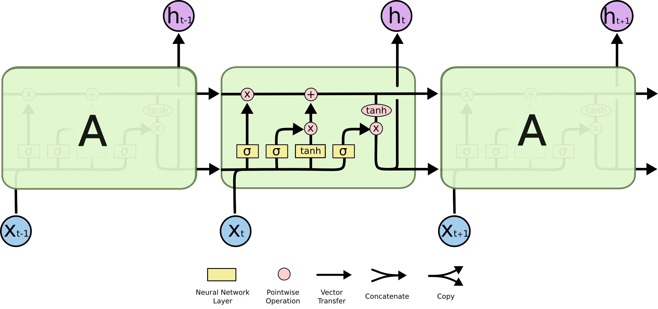
LSTM models were designed to improve the handling of long-term dependencies.
- What problem is LSTM trying to solve?
- What is the purpose of having a cell state?
- What is the intuitive role of a forget gate?
- What is the intuitive role of an input gate?
- What is the intuitive role of an output gate?
Exercise 14: Motivation for GRU
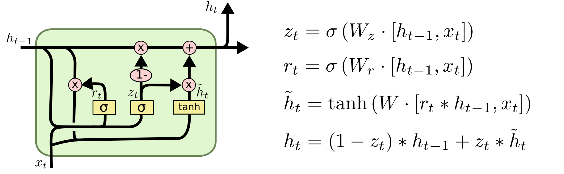
GRU is a simpler alternative to LSTM.
- What problem is GRU also trying to solve?
- How is GRU conceptually similar to LSTM?
- Why might GRU be faster to train than LSTM?
- In practice, why is it useful to compare SimpleRNN, LSTM and GRU rather than assuming one is always best?
Exercise 15: Comparing SimpleRNN, LSTM and GRU
Suppose you fit a SimpleRNN, an LSTM and a GRU to the same forecasting problem.
- Which model has the simplest recurrent structure?
- Which models are designed to better handle long-term dependence?
- Which model may have more parameters?
- What validation metric would you use for a regression forecasting problem?
- What validation metric would you use for a classification forecasting problem?
Part 6: Application: weather prediction with RNNs
In this section, we use weather prediction as a worked application of RNNs.
The goal is to practise the full modelling workflow for sequence data.
Exercise 16: Weather prediction as a sequence-modelling problem
Using the daily weather dataset, build and compare several models for predicting tomorrow’s weather class.
Follow the steps below.
Load the dataset and inspect the variables.
Identify the response variable and the available predictors.
Explain why this can be viewed as a sequence-modelling problem.
Split the data into training, validation and test sets using chronological order rather than random splitting.
Preprocess the predictors:
- scale the numerical variables;
- encode the categorical weather variable;
- make sure preprocessing is fitted using the training data only.
Create lagged sequence inputs.
For example, use the previous m days of observations to predict the weather class on the next day.Check the shape of the RNN input array.
Explain what each dimension represents in(\text{samples}, \text{time steps}, \text{features}).
Fit a simple baseline model, such as a majority-class or persistence baseline.
Fit a feedforward neural network using flattened lagged inputs.
Fit a SimpleRNN model using the sequence input.
Fit an LSTM model using the same sequence input.
Fit a GRU model using the same sequence input.
Compare the models using validation and test accuracy.
Plot or inspect the training histories of the neural-network models.
Discuss whether the recurrent models improve meaningfully over the simpler baselines.
Based on the results, decide which model you would choose for this application and justify your choice.