import os
os.environ["KERAS_BACKEND"] = "torch"

import keras
keras.utils.set_random_seed(1)Exercise: French Motor Claim Frequency
ACTL3143 & ACTL5111 Deep Learning for Actuaries
Your task is to predict the frequency distribution of car insurance claims in France.

French motor dataset
Show the package imports
import random
from pathlib import Path

import matplotlib.pyplot as plt
import numpy as np
import pandas as pd

import keras
from keras.callbacks import EarlyStopping
from keras.models import Sequential
from keras.layers import Dense

from sklearn.compose import make_column_transformer
from sklearn.datasets import fetch_openml
from sklearn.linear_model import LinearRegression
from sklearn.model_selection import train_test_split
from sklearn.preprocessing import OneHotEncoder, OrdinalEncoder, StandardScaler
from sklearn import set_config

import statsmodels.api as sm

set_config(transform_output="pandas")
Download the dataset if we don’t have it already.
- 1
- Checks if the dataset does not already exist within the Jupyter Notebook directory.
- 2
- Fetches the dataset from OpenML
- 3
-
Converts the dataset into
csvformat - 4
- If it already exists, then read in the dataset from the file.
| IDpol | ClaimNb | Exposure | Area | VehPower | VehAge | DrivAge | BonusMalus | VehBrand | VehGas | Density | Region | |
|---|---|---|---|---|---|---|---|---|---|---|---|---|
| 0 | 1.0 | 1.0 | 0.10000 | D | 5.0 | 0.0 | 55.0 | 50.0 | B12 | Regular | 1217.0 | R82 |
| 1 | 3.0 | 1.0 | 0.77000 | D | 5.0 | 0.0 | 55.0 | 50.0 | B12 | Regular | 1217.0 | R82 |
| 2 | 5.0 | 1.0 | 0.75000 | B | 6.0 | 2.0 | 52.0 | 50.0 | B12 | Diesel | 54.0 | R22 |
| 3 | 10.0 | 1.0 | 0.09000 | B | 7.0 | 0.0 | 46.0 | 50.0 | B12 | Diesel | 76.0 | R72 |
| 4 | 11.0 | 1.0 | 0.84000 | B | 7.0 | 0.0 | 46.0 | 50.0 | B12 | Diesel | 76.0 | R72 |
| ... | ... | ... | ... | ... | ... | ... | ... | ... | ... | ... | ... | ... |
| 678008 | 6114326.0 | 0.0 | 0.00274 | E | 4.0 | 0.0 | 54.0 | 50.0 | B12 | Regular | 3317.0 | R93 |
| 678009 | 6114327.0 | 0.0 | 0.00274 | E | 4.0 | 0.0 | 41.0 | 95.0 | B12 | Regular | 9850.0 | R11 |
| 678010 | 6114328.0 | 0.0 | 0.00274 | D | 6.0 | 2.0 | 45.0 | 50.0 | B12 | Diesel | 1323.0 | R82 |
| 678011 | 6114329.0 | 0.0 | 0.00274 | B | 4.0 | 0.0 | 60.0 | 50.0 | B12 | Regular | 95.0 | R26 |
| 678012 | 6114330.0 | 0.0 | 0.00274 | B | 7.0 | 6.0 | 29.0 | 54.0 | B12 | Diesel | 65.0 | R72 |
678013 rows × 12 columns
Data dictionary
IDpol: policy number (unique identifier)Area: area code (categorical, ordinal)BonusMalus: bonus-malus level between 50 and 230 (with reference level 100)Density: density of inhabitants per km2 in the city of the living place of the driverDrivAge: age of the (most common) driver in yearsExposure: total exposure in yearly unitsRegion: regions in France (prior to 2016)VehAge: age of the car in yearsVehBrand: car brand (categorical, nominal)VehGas: diesel or regular fuel car (binary)VehPower: power of the car (categorical, ordinal)ClaimNb: number of claims on the given policy (target variable)
Region column
Poisson regression
The model
Have \{ (\boldsymbol{x}_i, y_i) \}_{i=1, \dots, n} for \boldsymbol{x}_i \in \mathbb{R}^{47} and y_i \in \mathbb{N}_0.
Assume the distribution Y_i \sim \mathsf{Poisson}(\lambda(\boldsymbol{x}_i))
We have \mathbb{E} Y_i = \lambda(\boldsymbol{x}_i). The NN takes \boldsymbol{x}_i & predicts \mathbb{E} Y_i.
Note
For insurance, this is a bit weird. The exposures are different for each policy.
\lambda(\boldsymbol{x}_i) is the expected number of claims for the duration of policy i’s contract.
Normally, \text{Exposure}_i \not\in \boldsymbol{x}_i, and \lambda(\boldsymbol{x}_i) is the expected rate per year, then Y_i \sim \mathsf{Poisson}(\text{Exposure}_i \times \lambda(\boldsymbol{x}_i)).
Help about the “poisson” loss
help(keras.losses.poisson)Help on function poisson in module keras.src.losses.losses:
poisson(y_true, y_pred)
Computes the Poisson loss between y_true and y_pred.
Formula:
```python
loss = y_pred - y_true * log(y_pred)
```
Args:
y_true: Ground truth values. shape = `[batch_size, d0, .. dN]`.
y_pred: The predicted values. shape = `[batch_size, d0, .. dN]`.
Returns:
Poisson loss values with shape = `[batch_size, d0, .. dN-1]`.
Example:
>>> y_true = np.random.randint(0, 2, size=(2, 3))
>>> y_pred = np.random.random(size=(2, 3))
>>> loss = keras.losses.poisson(y_true, y_pred)
>>> assert loss.shape == (2,)
>>> y_pred = y_pred + 1e-7
>>> assert np.allclose(
... loss, np.mean(y_pred - y_true * np.log(y_pred), axis=-1),
... atol=1e-5)
Poisson probabilities
Since the probability mass function (p.m.f.) of the N \sim \mathsf{Poisson}(\lambda) distribution is \mathbb{P}(N = k) = \frac{\lambda^k \mathrm{e}^{-\lambda}}{k!} then the p.m.f. of Y_i \sim \mathsf{Poisson}(\lambda(\boldsymbol{x}_i)) is
\mathbb{P}(Y_i = y_i) = \frac{ \lambda(\boldsymbol{x}_i)^{y_i} \, \mathrm{e}^{-\lambda(\boldsymbol{x}_i)} }{y_i!}
The likelihood of a sample is then \mathbb{P}(Y_1 = y_1, \dots, Y_n = y_n) = \prod_{i=1}^n \mathbb{P}(Y_i = y_i).
Log-likelihood
Therefore, the likelihood of \{ (\boldsymbol{x}_i, y_i) \}_{i=1, \dots, n} is
L = \prod_{i=1}^n \frac{ \lambda(\boldsymbol{x}_i)^{y_i} \, \mathrm{e}^{-\lambda(\boldsymbol{x}_i)} }{y_i!}
so the log-likelihood is
\begin{aligned} \ell &= \sum_{i=1}^n \log \bigl( \frac{ \lambda(\boldsymbol{x}_i)^{y_i} \, \mathrm{e}^{-\lambda(\boldsymbol{x}_i)} }{y_i!} \bigr) \\ &= \sum_{i=1}^n y_i \log \bigl( \lambda(\boldsymbol{x}_i) \bigr) - \lambda(\boldsymbol{x}_i) - \log(y_i!) . \end{aligned}
Maximising the likelihood
Want to find the best NN \lambda^* such that: \begin{aligned} \lambda^* &= \arg\max_{\lambda} \sum_{i=1}^n y_i \log \bigl( \lambda(\boldsymbol{x}_i) \bigr) - \lambda(\boldsymbol{x}_i) - \log(y_i!) \\ &= \arg\max_{\lambda} \sum_{i=1}^n y_i \log \bigl( \lambda(\boldsymbol{x}_i) \bigr) - \lambda(\boldsymbol{x}_i) \\ &= \arg\min_{\lambda} \sum_{i=1}^n \lambda(\boldsymbol{x}_i) - y_i \log \bigl( \lambda(\boldsymbol{x}_i)\bigr) \\ &= \arg\min_{\lambda} \frac{1}{n} \sum_{i=1}^n \lambda(\boldsymbol{x}_i) - y_i \log \bigl( \lambda(\boldsymbol{x}_i)\bigr) . \end{aligned}
Keras’ “poisson” loss again
help(poisson)Help on function poisson in module keras.losses:
poisson(y_true, y_pred)
Computes the Poisson loss between y_true and y_pred.
The Poisson loss is the mean of the elements of the `Tensor`
`y_pred - y_true * log(y_pred)`.
...
In other words, \text{PoissonLoss} = \frac{1}{n} \sum_{i=1}^n \lambda(\boldsymbol{x}_i) - y_i \log \bigl( \lambda(\boldsymbol{x}_i) \bigr) .
Poisson deviance
D = 2 \sum_{i=1}^n y_i \log\bigl( \frac{y_i}{\lambda(\boldsymbol{x}_i)} \bigr) - \bigl( y_i - \lambda(\boldsymbol{x}_i) \bigr) .
from sklearn.metrics import mean_poisson_deviance
y_true = [0, 2, 1]
y_pred = [0.1, 0.9, 0.8]
mean_poisson_deviance(y_true, y_pred)0.4134392958331687deviance = 0
for y_i, yhat_i in zip(y_true, y_pred):
firstTerm = y_i * np.log(y_i / yhat_i) if y_i > 0 else 0
deviance += 2 * (firstTerm - (y_i - yhat_i))
meanDeviance = deviance / len(y_true)
deviance, meanDeviance(np.float64(1.240317887499506), np.float64(0.4134392958331687))Poisson deviance as a loss function
Want to find the best NN \lambda^* such that: \begin{aligned} \lambda^* &= \arg\min_{\lambda} \, 2 \sum_{i=1}^n y_i \log\bigl( \frac{y_i}{\lambda(\boldsymbol{x}_i)} \bigr) - \bigl( y_i - \lambda(\boldsymbol{x}_i) \bigr) \\ &= \arg\min_{\lambda} \sum_{i=1}^n y_i \log( y_i ) - y_i \log\bigl( \lambda(\boldsymbol{x}_i) \bigr) - y_i + \lambda(\boldsymbol{x}_i) \\ &= \arg\min_{\lambda} \sum_{i=1}^n - y_i \log\bigl( \lambda(\boldsymbol{x}_i) \bigr) + \lambda(\boldsymbol{x}_i) \\ &= \arg\min_{\lambda} \sum_{i=1}^n \lambda(\boldsymbol{x}_i) - y_i \log\bigl( \lambda(\boldsymbol{x}_i) \bigr) . \end{aligned}
GLM
Split the data
X = freq.drop(columns=["ClaimNb", "IDpol"])
y = freq["ClaimNb"]

X_main, X_test, y_main, y_test = train_test_split(X, y, test_size=0.2, random_state=42)
X_train, X_val, y_train, y_val = train_test_split(X_main, y_main, test_size=0.25, random_state=42)TODO: Modify this to do a stratified split. That is, the distribution of ClaimNb should be (about) the same in the training, validation, and test sets.
Preprocess the inputs for a GLM
ct_glm = make_column_transformer(
  (OrdinalEncoder(), ["Area"]),
1  (OneHotEncoder(sparse_output=False, drop="first"),
      ["VehGas", "VehBrand", "Region"]),
  remainder="passthrough",
  verbose_feature_names_out=False
)
2X_train_glm = sm.add_constant(ct_glm.fit_transform(X_train))
X_val_glm = sm.add_constant(ct_glm.transform(X_val))
X_test_glm = sm.add_constant(ct_glm.transform(X_test))

X_train_glm- 1
-
The
drop="first"parameter is used to avoid multicollinearity in the model. - 2
-
The
sm.add_constantfunction adds a column of ones to the input matrix.
| const | Area | VehGas_Regular | VehBrand_B10 | VehBrand_B11 | VehBrand_B12 | VehBrand_B13 | VehBrand_B14 | VehBrand_B2 | VehBrand_B3 | ... | Region_R83 | Region_R91 | Region_R93 | Region_R94 | Exposure | VehPower | VehAge | DrivAge | BonusMalus | Density | |
|---|---|---|---|---|---|---|---|---|---|---|---|---|---|---|---|---|---|---|---|---|---|
| 642604 | 1.0 | 3.0 | 0.0 | 0.0 | 0.0 | 1.0 | 0.0 | 0.0 | 0.0 | 0.0 | ... | 0.0 | 1.0 | 0.0 | 0.0 | 0.74 | 11.0 | 1.0 | 50.0 | 50.0 | 824.0 |
| 394020 | 1.0 | 0.0 | 0.0 | 0.0 | 0.0 | 0.0 | 0.0 | 0.0 | 1.0 | 0.0 | ... | 0.0 | 0.0 | 0.0 | 0.0 | 1.00 | 6.0 | 10.0 | 51.0 | 55.0 | 42.0 |
| 104966 | 1.0 | 3.0 | 1.0 | 0.0 | 0.0 | 0.0 | 0.0 | 0.0 | 1.0 | 0.0 | ... | 0.0 | 0.0 | 0.0 | 0.0 | 1.00 | 4.0 | 20.0 | 81.0 | 50.0 | 747.0 |
| 438856 | 1.0 | 0.0 | 0.0 | 0.0 | 0.0 | 1.0 | 0.0 | 0.0 | 0.0 | 0.0 | ... | 0.0 | 0.0 | 0.0 | 0.0 | 0.25 | 7.0 | 3.0 | 44.0 | 50.0 | 23.0 |
| 87109 | 1.0 | 3.0 | 1.0 | 0.0 | 0.0 | 1.0 | 0.0 | 0.0 | 0.0 | 0.0 | ... | 0.0 | 0.0 | 1.0 | 0.0 | 0.12 | 7.0 | 1.0 | 52.0 | 50.0 | 721.0 |
| ... | ... | ... | ... | ... | ... | ... | ... | ... | ... | ... | ... | ... | ... | ... | ... | ... | ... | ... | ... | ... | ... |
| 99179 | 1.0 | 2.0 | 1.0 | 0.0 | 0.0 | 0.0 | 0.0 | 0.0 | 0.0 | 0.0 | ... | 0.0 | 0.0 | 0.0 | 0.0 | 0.31 | 7.0 | 6.0 | 49.0 | 50.0 | 119.0 |
| 523093 | 1.0 | 4.0 | 0.0 | 0.0 | 0.0 | 1.0 | 0.0 | 0.0 | 0.0 | 0.0 | ... | 0.0 | 0.0 | 1.0 | 0.0 | 0.04 | 7.0 | 0.0 | 43.0 | 51.0 | 4762.0 |
| 143052 | 1.0 | 2.0 | 0.0 | 0.0 | 0.0 | 0.0 | 1.0 | 0.0 | 0.0 | 0.0 | ... | 0.0 | 0.0 | 0.0 | 0.0 | 1.00 | 6.0 | 6.0 | 36.0 | 50.0 | 133.0 |
| 606805 | 1.0 | 1.0 | 0.0 | 0.0 | 0.0 | 1.0 | 0.0 | 0.0 | 0.0 | 0.0 | ... | 0.0 | 0.0 | 0.0 | 0.0 | 0.48 | 5.0 | 0.0 | 73.0 | 50.0 | 79.0 |
| 228897 | 1.0 | 0.0 | 1.0 | 0.0 | 0.0 | 0.0 | 0.0 | 0.0 | 0.0 | 1.0 | ... | 0.0 | 0.0 | 1.0 | 0.0 | 1.00 | 4.0 | 5.0 | 76.0 | 50.0 | 34.0 |
406807 rows × 40 columns
Alternatively, you can try to reproduce this using the patsy library and an R-style formula.
Fit a GLM
Using the statsmodels package, we can fit a Poisson regression model.
glm = sm.GLM(y_train, X_train_glm, family=sm.families.Poisson())
glm_results = glm.fit()
glm_results.summary()| Dep. Variable: | ClaimNb | No. Observations: | 406807 |
|---|---|---|---|
| Model: | GLM | Df Residuals: | 406767 |
| Model Family: | Poisson | Df Model: | 39 |
| Link Function: | Log | Scale: | 1.0000 |
| Method: | IRLS | Log-Likelihood: | -83303. |
| Date: | Wed, 01 Jul 2026 | Deviance: | 1.2522e+05 |
| Time: | 21:44:49 | Pearson chi2: | 4.56e+05 |
| No. Iterations: | 7 | Pseudo R-squ. (CS): | 0.01256 |
| Covariance Type: | nonrobust |
| coef | std err | z | P>|z| | [0.025 | 0.975] | |
|---|---|---|---|---|---|---|
| const | -5.2621 | 0.061 | -86.094 | 0.000 | -5.382 | -5.142 |
| Area | 0.0529 | 0.007 | 7.852 | 0.000 | 0.040 | 0.066 |
| VehGas_Regular | 0.0779 | 0.014 | 5.497 | 0.000 | 0.050 | 0.106 |
| VehBrand_B10 | -0.0629 | 0.049 | -1.296 | 0.195 | -0.158 | 0.032 |
| VehBrand_B11 | -0.0238 | 0.053 | -0.450 | 0.653 | -0.128 | 0.080 |
| VehBrand_B12 | 0.0577 | 0.023 | 2.528 | 0.011 | 0.013 | 0.103 |
| VehBrand_B13 | 0.0137 | 0.053 | 0.257 | 0.797 | -0.091 | 0.118 |
| VehBrand_B14 | -0.2025 | 0.104 | -1.943 | 0.052 | -0.407 | 0.002 |
| VehBrand_B2 | -0.0017 | 0.020 | -0.085 | 0.932 | -0.040 | 0.037 |
| VehBrand_B3 | -0.0357 | 0.029 | -1.250 | 0.211 | -0.092 | 0.020 |
| VehBrand_B4 | -0.0373 | 0.039 | -0.968 | 0.333 | -0.113 | 0.038 |
| VehBrand_B5 | 0.0837 | 0.032 | 2.620 | 0.009 | 0.021 | 0.146 |
| VehBrand_B6 | -0.0441 | 0.036 | -1.208 | 0.227 | -0.116 | 0.027 |
| Region_R21 | 0.0675 | 0.108 | 0.628 | 0.530 | -0.143 | 0.278 |
| Region_R22 | 0.0905 | 0.066 | 1.363 | 0.173 | -0.040 | 0.221 |
| Region_R23 | -0.1839 | 0.078 | -2.368 | 0.018 | -0.336 | -0.032 |
| Region_R24 | 0.1573 | 0.032 | 4.975 | 0.000 | 0.095 | 0.219 |
| Region_R25 | 0.0126 | 0.060 | 0.210 | 0.833 | -0.105 | 0.130 |
| Region_R26 | -0.0466 | 0.064 | -0.725 | 0.469 | -0.173 | 0.079 |
| Region_R31 | -0.0591 | 0.044 | -1.332 | 0.183 | -0.146 | 0.028 |
| Region_R41 | -0.2423 | 0.061 | -3.997 | 0.000 | -0.361 | -0.123 |
| Region_R42 | 0.0151 | 0.118 | 0.128 | 0.898 | -0.216 | 0.247 |
| Region_R43 | -0.0340 | 0.171 | -0.199 | 0.842 | -0.369 | 0.301 |
| Region_R52 | 0.0445 | 0.039 | 1.136 | 0.256 | -0.032 | 0.121 |
| Region_R53 | 0.1868 | 0.037 | 5.031 | 0.000 | 0.114 | 0.260 |
| Region_R54 | 0.0046 | 0.050 | 0.091 | 0.927 | -0.094 | 0.103 |
| Region_R72 | -0.1490 | 0.044 | -3.364 | 0.001 | -0.236 | -0.062 |
| Region_R73 | -0.1302 | 0.055 | -2.358 | 0.018 | -0.238 | -0.022 |
| Region_R74 | 0.2443 | 0.084 | 2.901 | 0.004 | 0.079 | 0.409 |
| Region_R82 | 0.1525 | 0.031 | 4.972 | 0.000 | 0.092 | 0.213 |
| Region_R83 | -0.2533 | 0.096 | -2.627 | 0.009 | -0.442 | -0.064 |
| Region_R91 | -0.0782 | 0.042 | -1.849 | 0.064 | -0.161 | 0.005 |
| Region_R93 | 0.0007 | 0.032 | 0.022 | 0.983 | -0.063 | 0.064 |
| Region_R94 | 0.1519 | 0.085 | 1.790 | 0.074 | -0.014 | 0.318 |
| Exposure | 1.0462 | 0.021 | 49.448 | 0.000 | 1.005 | 1.088 |
| VehPower | 0.0097 | 0.004 | 2.733 | 0.006 | 0.003 | 0.017 |
| VehAge | -0.0350 | 0.001 | -23.398 | 0.000 | -0.038 | -0.032 |
| DrivAge | 0.0091 | 0.001 | 17.680 | 0.000 | 0.008 | 0.010 |
| BonusMalus | 0.0202 | 0.000 | 49.319 | 0.000 | 0.019 | 0.021 |
| Density | -8.998e-07 | 2.22e-06 | -0.406 | 0.685 | -5.25e-06 | 3.45e-06 |
Extract the Poisson deviance from the GLM
glm_results.deviancenp.float64(125222.6772692274)Mean Poisson deviance:
glm_results.deviance / len(y_train)np.float64(0.30781839365897684)Using the mean_poisson_deviance function:
mean_poisson_deviance(y_train, glm_results.predict(X_train_glm))0.30781839365897684Validation set mean Poisson deviance:
mean_poisson_deviance(y_val, glm_results.predict(X_val_glm))0.3091974082275945TODO: Add in lasso or ridge regularization to the GLM using the validation set.
Neural network
Look at the counts of the Region and VehBrand columns
freq["Region"].value_counts().plot(kind="bar")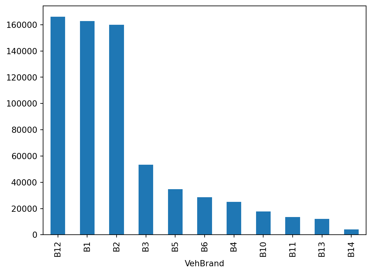
freq["VehBrand"].value_counts().plot(kind="bar")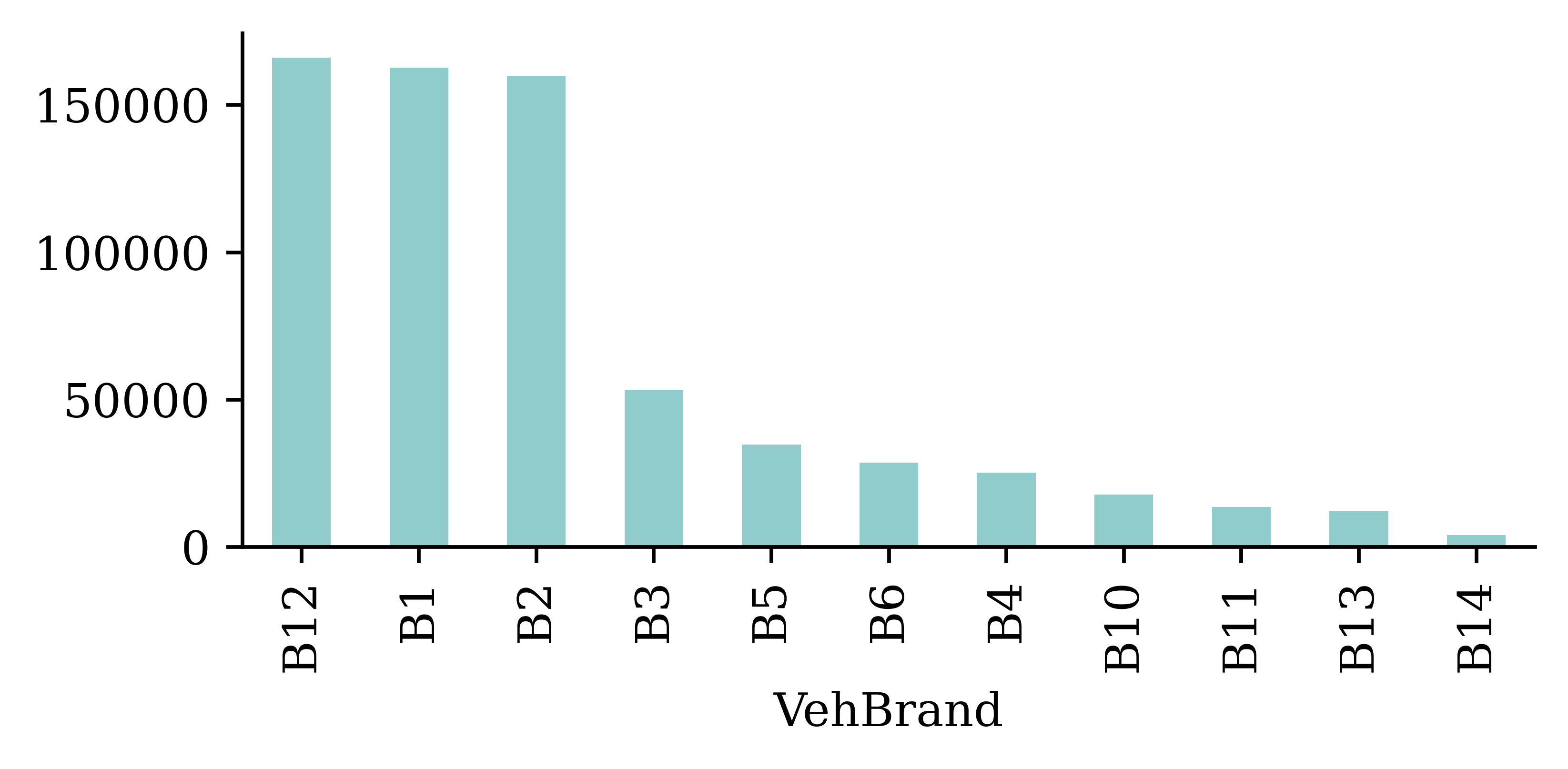
TODO: Consider combining the least frequent categories into a single category. That would reduce the cardinality of the categorical columns, and hence the number of input features.
Prepare the data for a neural network
ct = make_column_transformer(
  (OrdinalEncoder(), ["Area"]),
1  (OneHotEncoder(sparse_output=False, drop="if_binary"),
      ["VehGas", "VehBrand", "Region"]),
  remainder=StandardScaler(),
  verbose_feature_names_out=False
)
X_train_ct = ct.fit_transform(X_train)
X_val_ct = ct.transform(X_val)
X_test_ct = ct.transform(X_test)

X_train_ct- 1
-
The
drop="if_binary"parameter will only drop the first column if the column is binary (i.e. for theVehGascolumn).
| Area | VehGas_Regular | VehBrand_B1 | VehBrand_B10 | VehBrand_B11 | VehBrand_B12 | VehBrand_B13 | VehBrand_B14 | VehBrand_B2 | VehBrand_B3 | ... | Region_R83 | Region_R91 | Region_R93 | Region_R94 | Exposure | VehPower | VehAge | DrivAge | BonusMalus | Density | |
|---|---|---|---|---|---|---|---|---|---|---|---|---|---|---|---|---|---|---|---|---|---|
| 642604 | 3.0 | 0.0 | 0.0 | 0.0 | 0.0 | 1.0 | 0.0 | 0.0 | 0.0 | 0.0 | ... | 0.0 | 1.0 | 0.0 | 0.0 | 0.579995 | 2.216304 | -1.068169 | 0.319694 | -0.623906 | -0.244407 |
| 394020 | 0.0 | 0.0 | 0.0 | 0.0 | 0.0 | 0.0 | 0.0 | 0.0 | 1.0 | 0.0 | ... | 0.0 | 0.0 | 0.0 | 0.0 | 1.293590 | -0.221879 | 0.522740 | 0.390412 | -0.304423 | -0.441611 |
| 104966 | 3.0 | 1.0 | 0.0 | 0.0 | 0.0 | 0.0 | 0.0 | 0.0 | 1.0 | 0.0 | ... | 0.0 | 0.0 | 0.0 | 0.0 | 1.293590 | -1.197153 | 2.290416 | 2.511980 | -0.623906 | -0.263825 |
| 438856 | 0.0 | 0.0 | 0.0 | 0.0 | 0.0 | 1.0 | 0.0 | 0.0 | 0.0 | 0.0 | ... | 0.0 | 0.0 | 0.0 | 0.0 | -0.764858 | 0.265757 | -0.714634 | -0.104620 | -0.623906 | -0.446403 |
| 87109 | 3.0 | 1.0 | 0.0 | 0.0 | 0.0 | 1.0 | 0.0 | 0.0 | 0.0 | 0.0 | ... | 0.0 | 0.0 | 1.0 | 0.0 | -1.121655 | 0.265757 | -1.068169 | 0.461131 | -0.623906 | -0.270382 |
| ... | ... | ... | ... | ... | ... | ... | ... | ... | ... | ... | ... | ... | ... | ... | ... | ... | ... | ... | ... | ... | ... |
| 99179 | 2.0 | 1.0 | 1.0 | 0.0 | 0.0 | 0.0 | 0.0 | 0.0 | 0.0 | 0.0 | ... | 0.0 | 0.0 | 0.0 | 0.0 | -0.600182 | 0.265757 | -0.184331 | 0.248975 | -0.623906 | -0.422194 |
| 523093 | 4.0 | 0.0 | 0.0 | 0.0 | 0.0 | 1.0 | 0.0 | 0.0 | 0.0 | 0.0 | ... | 0.0 | 0.0 | 1.0 | 0.0 | -1.341223 | 0.265757 | -1.244937 | -0.175339 | -0.560009 | 0.748673 |
| 143052 | 2.0 | 0.0 | 0.0 | 0.0 | 0.0 | 0.0 | 1.0 | 0.0 | 0.0 | 0.0 | ... | 0.0 | 0.0 | 0.0 | 0.0 | 1.293590 | -0.221879 | -0.184331 | -0.670371 | -0.623906 | -0.418663 |
| 606805 | 1.0 | 0.0 | 0.0 | 0.0 | 0.0 | 1.0 | 0.0 | 0.0 | 0.0 | 0.0 | ... | 0.0 | 0.0 | 0.0 | 0.0 | -0.133600 | -0.709516 | -1.244937 | 1.946228 | -0.623906 | -0.432281 |
| 228897 | 0.0 | 1.0 | 0.0 | 0.0 | 0.0 | 0.0 | 0.0 | 0.0 | 0.0 | 1.0 | ... | 0.0 | 0.0 | 1.0 | 0.0 | 1.293590 | -1.197153 | -0.361099 | 2.158385 | -0.623906 | -0.443629 |
406807 rows × 41 columns
Fit a neural network
model = Sequential([
    Dense(64, activation='leaky_relu', input_shape=(X_train_ct.shape[1],)),
    Dense(32, activation='leaky_relu'),
    Dense(1, activation='exponential')
])

model.compile(optimizer='adam', loss='poisson')
es = EarlyStopping(patience=5, restore_best_weights=True)
history = model.fit(X_train_ct, y_train, validation_data=(X_val_ct, y_val), epochs=100, batch_size=2048, callbacks=[es], verbose=0)Evaluate
model.evaluate(X_train_ct, y_train, verbose=0)0.19554777443408966y_train_pred = model.predict(X_train_ct, verbose=0)
mean_poisson_deviance(y_train, y_train_pred)0.29403199881392694y_val_pred = model.predict(X_val_ct, verbose=0)
mean_poisson_deviance(y_val, y_val_pred)0.29894756124339095TODO: Change exposure to be an offset in the Poisson regression model, both in the GLM and the neural network.