Time Series & Recurrent Neural Networks

ACTL3143 & ACTL5111 Deep Learning for Actuaries

Author

Patrick Laub

Show the package imports

import random
from pathlib import Path

import matplotlib.pyplot as plt
import numpy as np
import pandas as pd

from sklearn.linear_model import LinearRegression
from sklearn.metrics import mean_squared_error

from keras.models import Sequential
from keras.layers import Dense, Input, Rescaling
from keras.callbacks import EarlyStopping

Time Series

Tabular data vs time series data

Tabular data

We have a dataset \{ \boldsymbol{x}_i, y_i \}_{i=1}^n which we assume are i.i.d. observations.

Brand	Mileage	# Claims
BMW	101 km	1
Audi	432 km	0
Volvo	3 km	5
\vdots	\vdots	\vdots

The goal is to predict the y for some covariates \boldsymbol{x}.

Time series data

Have a sequence \{ \boldsymbol{x}_t, y_t \}_{t=1}^T of observations taken at regular time intervals.

Date	Humidity	Temp.
Jan 1	60%	20 °C
Jan 2	65%	22 °C
Jan 3	70%	21 °C
\vdots	\vdots	\vdots

The task is to forecast future values based on the past.

Attributes of time series data

Temporal ordering: The order of the observations matters.
Trend: The general direction of the data.
Noise: Random fluctuations in the data.
Seasonality: Patterns that repeat at regular intervals.

Question

What will be the temperature in Berlin tomorrow? What information would you use to make a prediction?

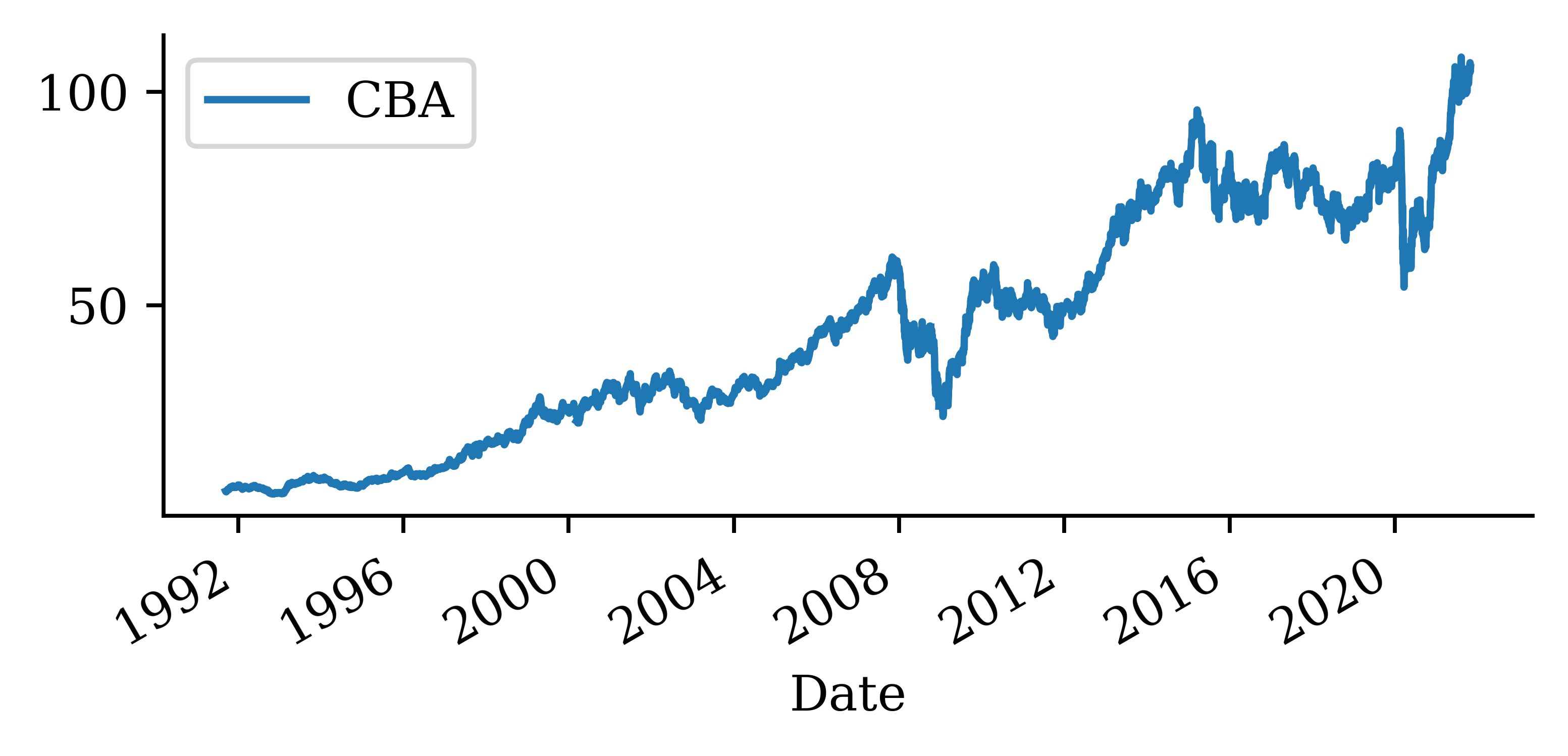
Australian financial stocks

# First, install yfinance if you haven't already:
# pip install yfinance
import yfinance as yf
import pandas as pd
from datetime import date

# 1. Define the ASX tickers (Yahoo uses “.AX” for Australian stocks
#    and “^AXJO” for the S&P/ASX 200 index)
tickers = {
    "ANZ":    "ANZ.AX",
    "BOQ":    "BOQ.AX",
    "CBA":    "CBA.AX",
    "NAB":    "NAB.AX",
    "QBE":    "QBE.AX",
    "SUN":    "SUN.AX",
    "WBC":    "WBC.AX",
    "ASX200": "^AXJO"
}

# 2. Choose your date range
start = "1999-01-01"
end   = date.today().isoformat()  # e.g. "2025-06-29"

# 3. Download the data
#    This returns a Panel-like DataFrame: columns are tickers, rows are trading dates.
raw_data = yf.download(
    tickers=list(tickers.values()),
    start=start,
    end=end,
    progress=False
)

raw_data.to_csv("asx_raw_data.csv")  # Optional: Save raw data for inspection

data = raw_data["Close"]

# 4. Rename columns to the simple names
data.rename(columns={v: k for k, v in tickers.items()}, inplace=True)

cols = ["ANZ", "ASX200", "BOQ", "CBA", "NAB", "QBE", "SUN", "WBC"]
data = data[cols]

# 5. (Optional) Inspect the first few rows
print(data.head())

# 6. Save to CSV
output_path = "aus_fin_stocks.csv"
data.to_csv(output_path)
print(f"Saved daily close prices to {output_path}")

Australian financial stocks

stocks = pd.read_csv("aus_fin_stocks.csv")
stocks

	Date	ANZ	ASX200	BOQ	CBA	NAB	QBE	SUN	WBC
0	1999-01-01	8.413491	NaN	NaN	14.560169	NaN	NaN	7.965791	NaN
1	1999-01-04	8.476515	2732.199951	NaN	14.402927	12.995510	2.648447	7.965791	6.370629
2	1999-01-05	8.452881	2716.600098	NaN	14.409224	13.169948	2.564247	7.965791	6.485921
...	...	...	...	...	...	...	...	...	...
6742	2025-06-25	29.100000	8559.200195	7.86	191.399994	40.049999	23.480000	21.750000	34.540001
6743	2025-06-26	29.740000	8550.799805	7.86	190.710007	39.889999	23.330000	21.459999	34.570000
6744	2025-06-27	29.200001	8514.200195	7.77	185.360001	39.259998	23.219999	21.330000	33.900002

6745 rows × 9 columns

Plot

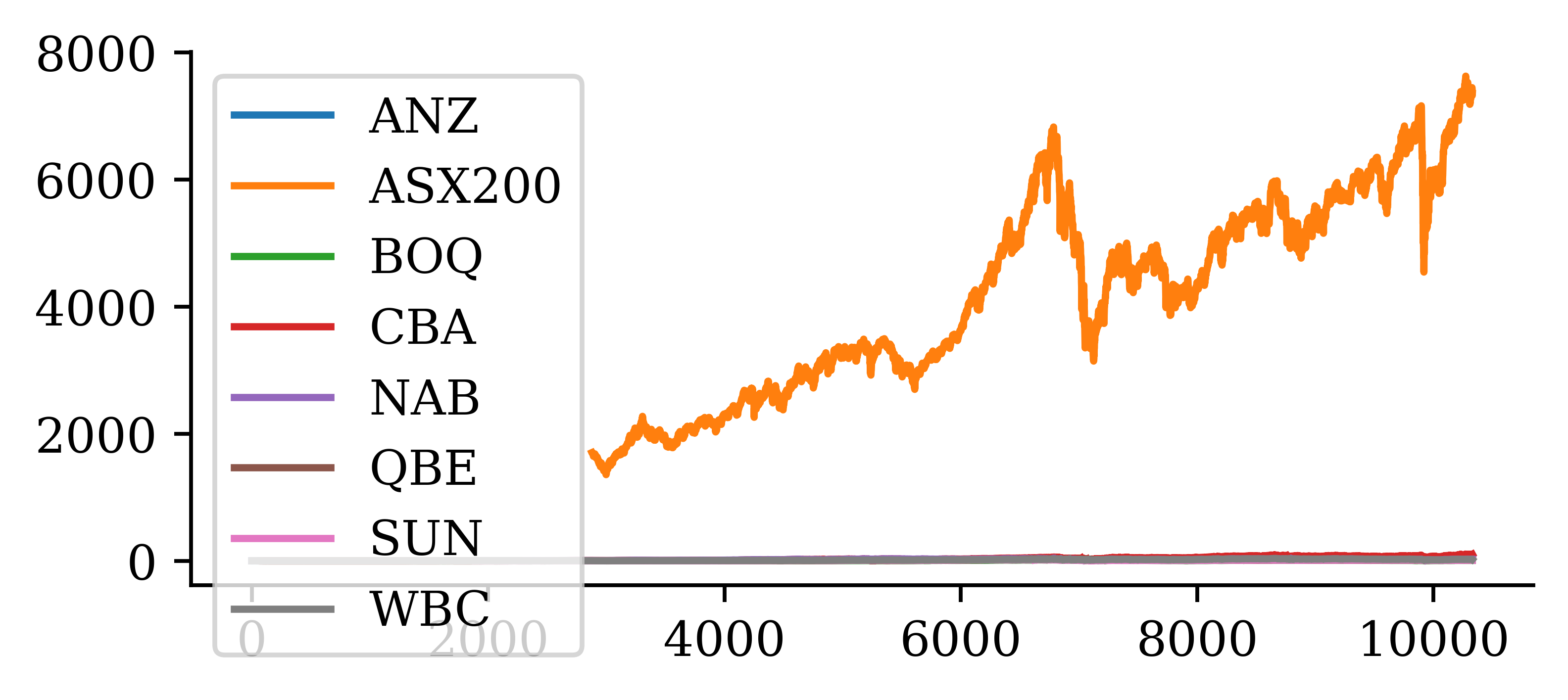
stocks.plot()

Question

What is wrong with this plot?

Answer: The main issues are * x-axis is unclear: should show the date, not the observation number * The ASX200 has much larger value than the individual stocks; it should be plotted separately. * The legend shouldn’t be overlapping and hiding half of the plot.

Data types and NA values

stocks.info()

<class 'pandas.DataFrame'>
RangeIndex: 6745 entries, 0 to 6744
Data columns (total 9 columns):
 #   Column  Non-Null Count  Dtype  
---  ------  --------------  -----  
 0   Date    6745 non-null   str    
 1   ANZ     6745 non-null   float64
 2   ASX200  6691 non-null   float64
 3   BOQ     6599 non-null   float64
 4   CBA     6745 non-null   float64
 5   NAB     6744 non-null   float64
 6   QBE     6744 non-null   float64
 7   SUN     6745 non-null   float64
 8   WBC     6744 non-null   float64
dtypes: float64(8), str(1)
memory usage: 540.3 KB

for col in stocks.columns:
    print(f"{col}: {stocks[col].isna().sum()}")

Date: 0
ANZ: 0
ASX200: 54
BOQ: 146
CBA: 0
NAB: 1
QBE: 1
SUN: 0
WBC: 1

asx200 = stocks.pop("ASX200")

Set the index to the date

stocks["Date"] = pd.to_datetime(stocks["Date"])
stocks = stocks.set_index("Date") # or `stocks.set_index("Date", inplace=True)`
stocks

	ANZ	BOQ	CBA	NAB	QBE	SUN	WBC
Date
1999-01-01	8.413491	NaN	14.560169	NaN	NaN	7.965791	NaN
1999-01-04	8.476515	NaN	14.402927	12.995510	2.648447	7.965791	6.370629
1999-01-05	8.452881	NaN	14.409224	13.169948	2.564247	7.965791	6.485921
...	...	...	...	...	...	...	...
2025-06-25	29.100000	7.86	191.399994	40.049999	23.480000	21.750000	34.540001
2025-06-26	29.740000	7.86	190.710007	39.889999	23.330000	21.459999	34.570000
2025-06-27	29.200001	7.77	185.360001	39.259998	23.219999	21.330000	33.900002

6745 rows × 7 columns

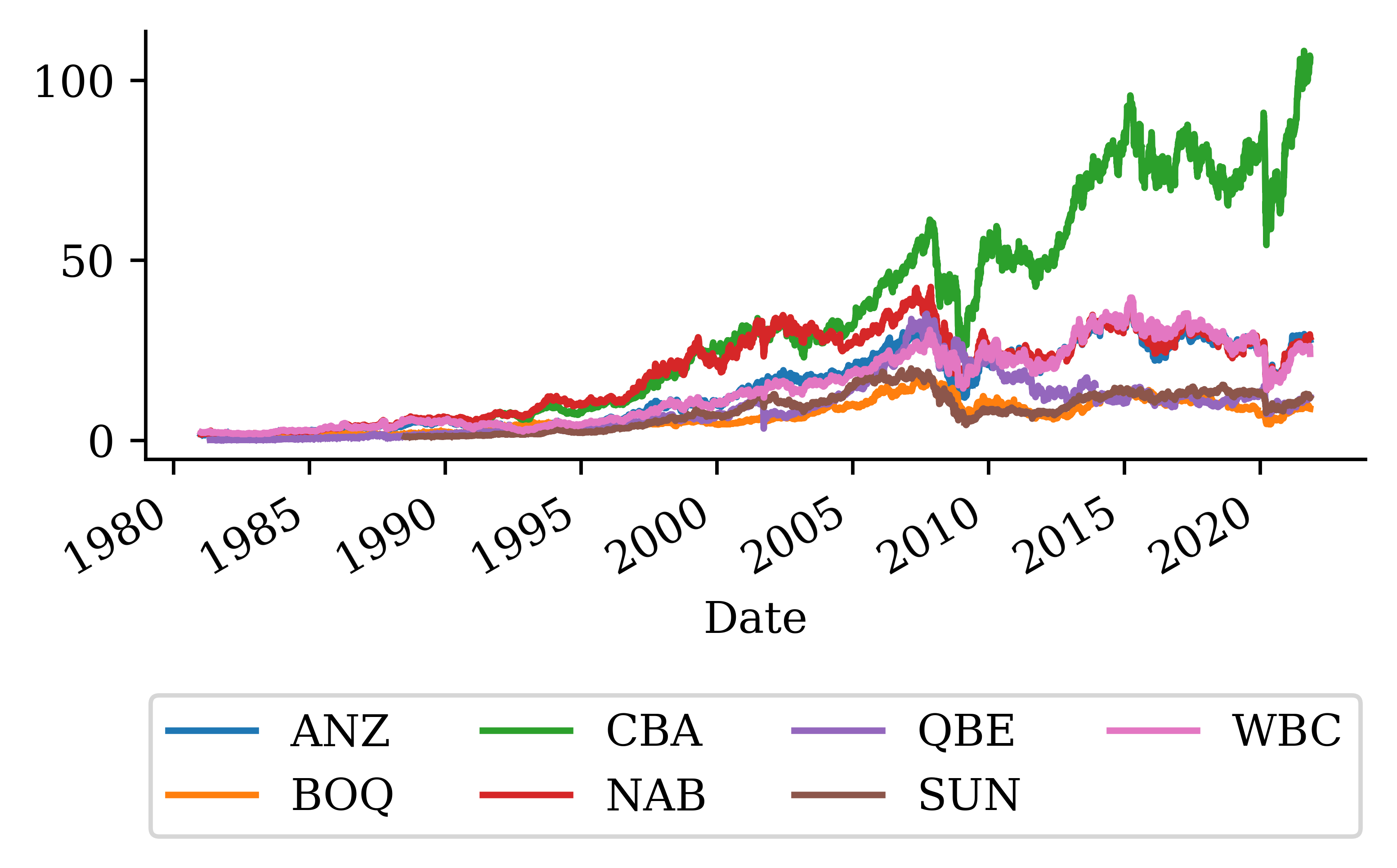
By setting the index to the date (and converting the date to a proper date format rather than a string), the plot of the stocks can be updated accordingly very easily.

Plot II

stocks.plot()
plt.ylabel("Stock Price ($)")
plt.legend(loc="upper center", bbox_to_anchor=(0.5, -0.5), ncol=4);

Can index using dates I

We can filter our data nicely using the dates that are now indexed.

stocks.loc["2010-1-4":"2010-01-8"]

	ANZ	BOQ	CBA	NAB	QBE	SUN	WBC
Date
2010-01-04	18.874071	8.412694	34.510429	14.440043	13.831507	10.478957	14.958415
2010-01-05	18.964771	8.520640	35.032455	14.624498	13.902833	10.636262	15.082577
2010-01-06	18.684425	8.477461	35.208561	14.339908	13.688861	10.406354	15.011630
2010-01-07	18.239164	8.218388	34.868923	14.223969	13.441965	10.551559	14.810603
2010-01-08	18.346357	8.419890	35.321777	14.176538	13.590102	10.612061	14.869730

Note, these ranges are inclusive, not like Python’s normal slicing.

Can index using dates II

So to get 2019’s December and all of 2020 for CBA:

stocks.loc["2019-12":"2020", ["CBA"]]

	CBA
Date
2019-12-02	66.193298
2019-12-03	64.494362
2019-12-04	63.250660
...	...
2020-12-29	70.822792
2020-12-30	70.468712
2020-12-31	69.221031

275 rows × 1 columns

Can look at the first differences

Rather than looking directly at the time series, we can remove the effect of the trend by looking at first differences.

stocks.diff().plot()
plt.ylabel("Daily Price Changes ($)")
plt.legend(loc="upper center", bbox_to_anchor=(0.5, -0.5), ncol=4);

The variance of the first differences increases over time (heteroscedasticity). This is a natural occurrence when the stock price increases over time.

Can look at the percentage changes

We can normalise the differences by taking the percentage changes.

stocks.pct_change().plot()
plt.ylabel("Daily Returns (%)")
plt.legend(loc="upper center", bbox_to_anchor=(0.5, -0.5), ncol=4);

Focus on one stock

stock = stocks[["CBA"]].copy()
stock

	CBA
Date
1999-01-01	14.560169
1999-01-04	14.402927
1999-01-05	14.409224
...	...
2025-06-25	191.399994
2025-06-26	190.710007
2025-06-27	185.360001

6745 rows × 1 columns

stock.plot()
plt.ylabel("Stock Price ($)");

stock.isna().sum()

CBA    0
dtype: int64

Convert to log returns

Instead of working with raw prices, we’ll work with daily log returns:

# Calculate log returns
stock_log = np.log(stock / stock.shift(1)).dropna()
stock_log.head()

	CBA
Date
1999-01-04	-0.010858
1999-01-05	0.000437
1999-01-06	0.008042
1999-01-07	0.025859
1999-01-08	-0.021323

Code

stock_log.plot()
plt.ylabel("Daily Log Return")
plt.title("CBA Daily Log Returns");

Code

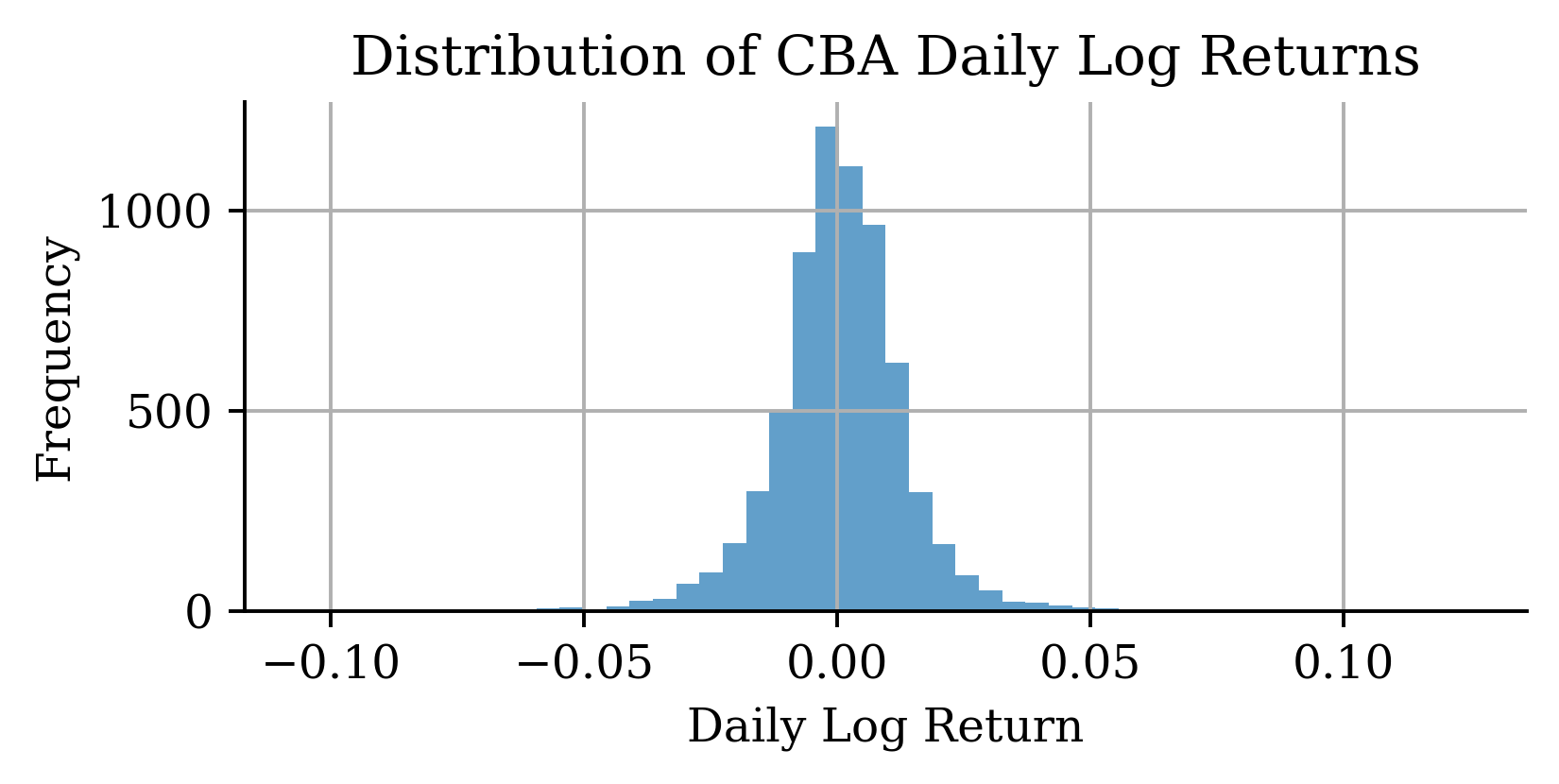
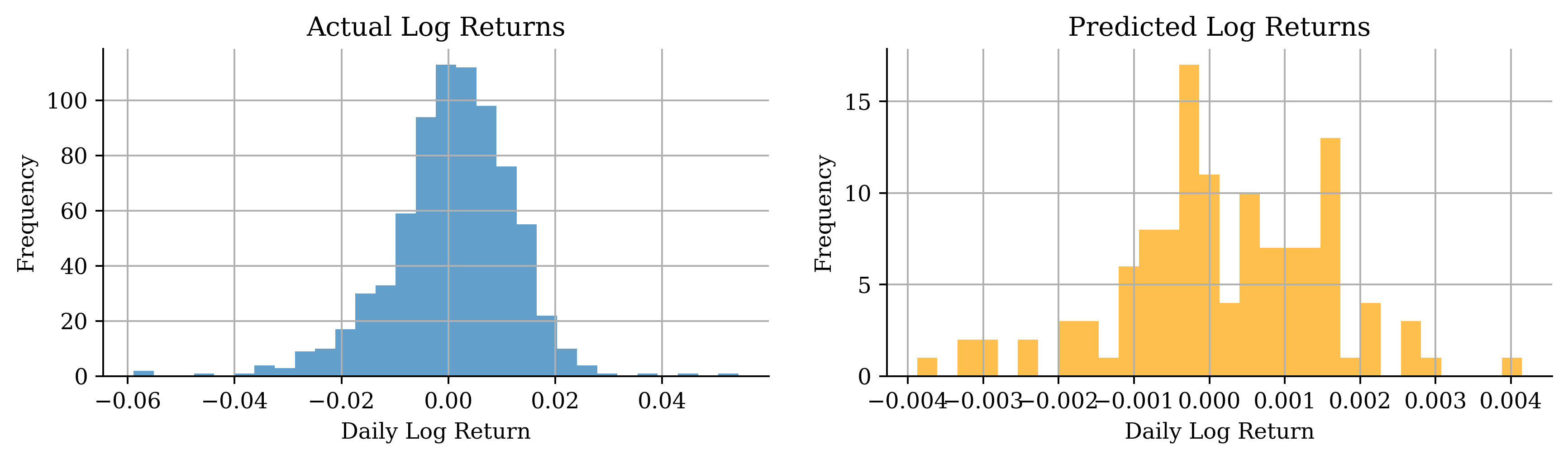
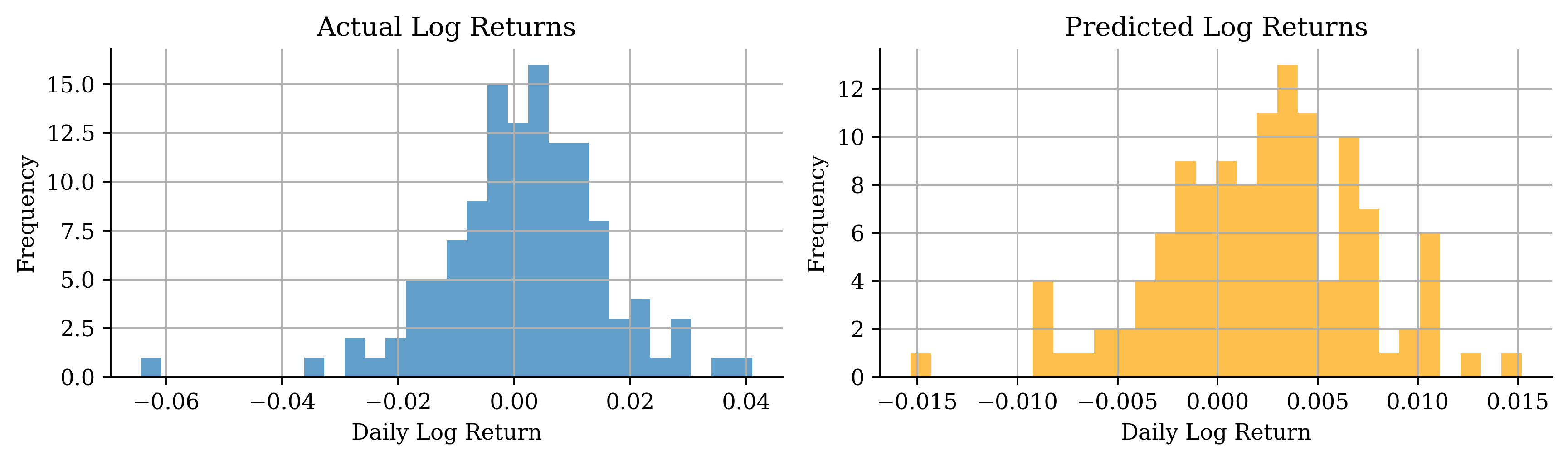
# Distribution of log returns
stock_log.hist(bins=50, alpha=0.7)
plt.xlabel("Daily Log Return")
plt.ylabel("Frequency")
plt.title("Distribution of CBA Daily Log Returns");

Fill in the missing values

Some of the data has missing values. Here, we fill in the missing values by taking the value from the previous day. If the previous day also has missing value, then you do the same thing until all values are filled. This is called foward-filling.

asx200 = pd.DataFrame(asx200).set_index(stocks.index)
missing_day = asx200.index[asx200["ASX200"].isna()][1]
prev_day = missing_day - pd.Timedelta(days=1)
after = missing_day + pd.Timedelta(days=3)

asx200.loc[prev_day:after]

	ASX200
Date
1999-01-25	2713.100098
1999-01-26	NaN
1999-01-27	2738.800049
1999-01-28	2765.100098
1999-01-29	2781.699951

asx200 = asx200.ffill()
asx200.loc[prev_day:after]

	ASX200
Date
1999-01-25	2713.100098
1999-01-26	2713.100098
1999-01-27	2738.800049
1999-01-28	2765.100098
1999-01-29	2781.699951

Baseline forecasts

We look at some baseline forecast methods.

Helper functions

def log_to_price(log_returns, initial_price):
    """Convert log returns to raw prices given an initial price."""
    # Use cumulative sum of log returns for numerical stability
    # P_t = P_0 * exp(sum of log returns from 1 to t)
    cumulative_log_returns = log_returns.cumsum()
    prices = initial_price * np.exp(cumulative_log_returns)
    
    return prices

def get_last_price(stock_df, cutoff_date):
    """Get the last known price before the forecast period starts."""
    last_known_date = stock_df.loc[:cutoff_date].index[-1]
    return stock_df.loc[last_known_date, "CBA"]

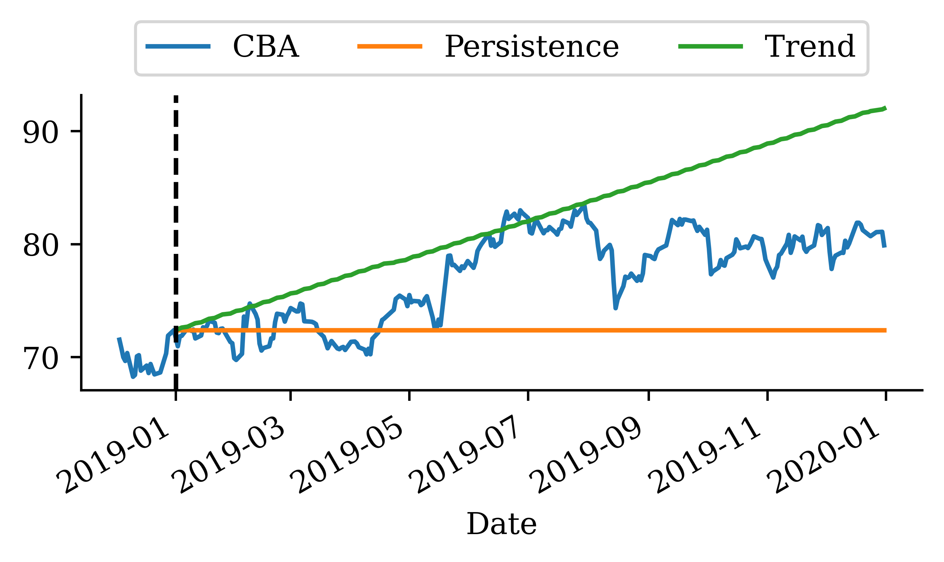
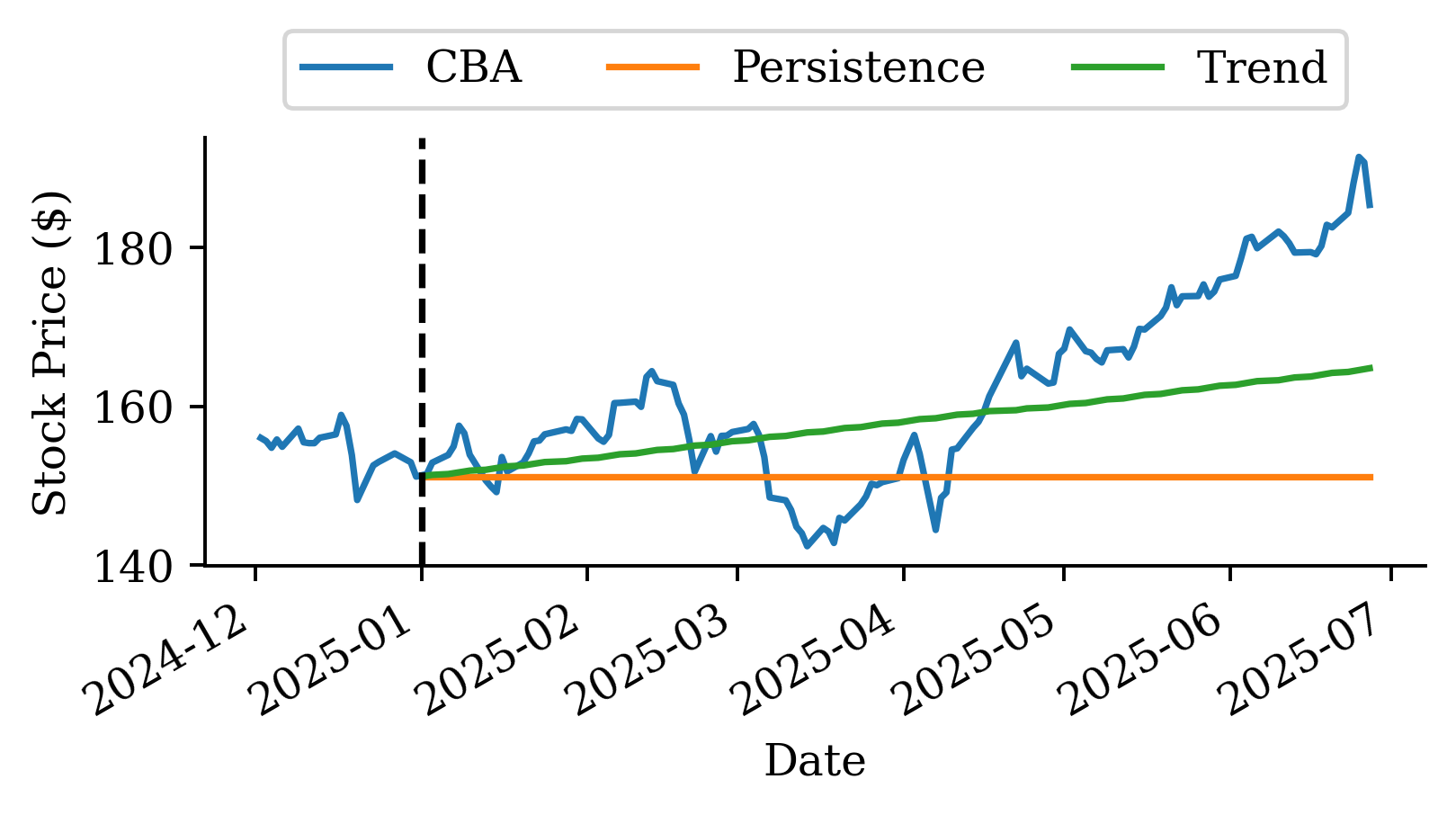
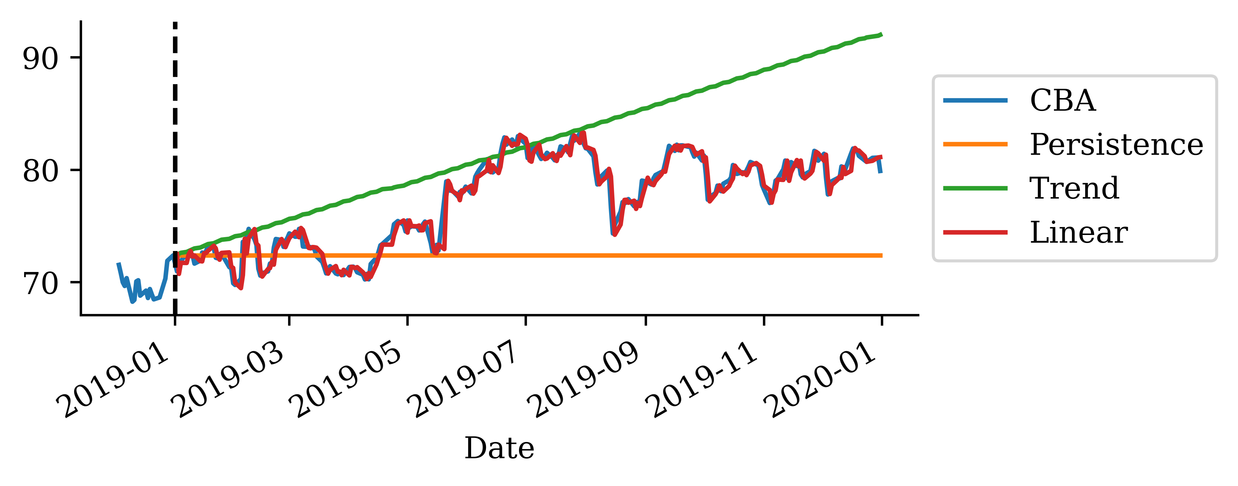
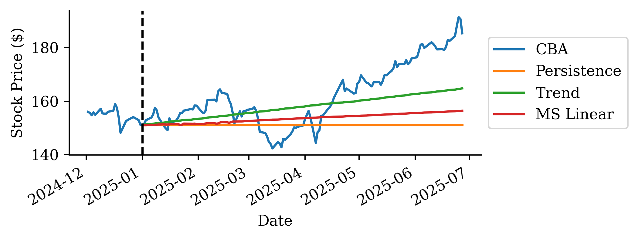
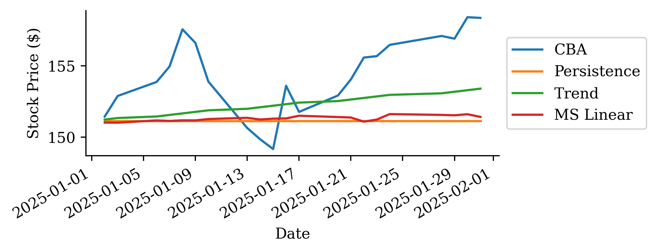
Persistence forecast

Predict the next value to be the same as the current value.

last_price = get_last_price(stock, cutoff_date="2024-12")
log_persistence = pd.Series(0.0, index=stock_log.loc["2025":].index)
persistence_prices = log_to_price(log_persistence, last_price)

Code

start = "2024-12"
end = "2025"
stock.loc[start:end, ["CBA"]].plot(label="CBA")
persistence_prices.plot(label="Persistence")
plt.axvline("2025-01", color="black", linestyle="--")
plt.ylabel("Stock Price ($)")
plt.legend()

Extrapolate the trend

recent_log_returns = stock_log.loc["2022-01":"2024-12"]
trend_log = recent_log_returns.mean().values[0]
print(f"Average daily log return: {trend_log:.6f}")

Average daily log return: 0.000709

log_trend = pd.Series(trend_log, index=stock_log.loc["2025":].index)
trend_prices = log_to_price(log_trend, last_price)

Code

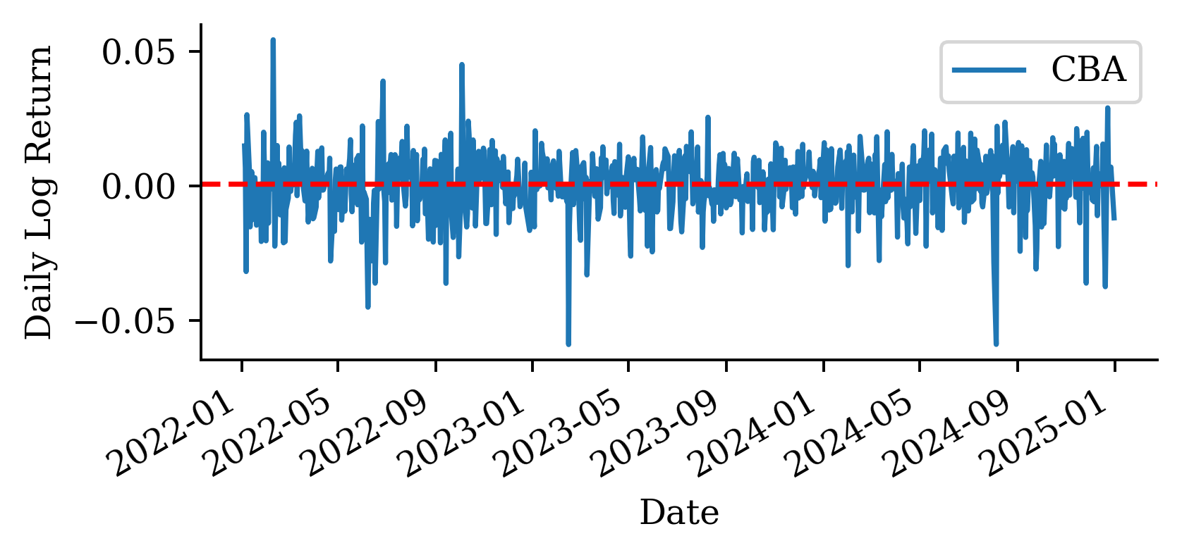
# Plot the trend line over the top of the 'recent_log_returns' data
recent_log_returns.plot()
plt.axhline(trend_log, color="red", linestyle="--", label="Trend (mean log return)")
plt.ylabel("Daily Log Return");

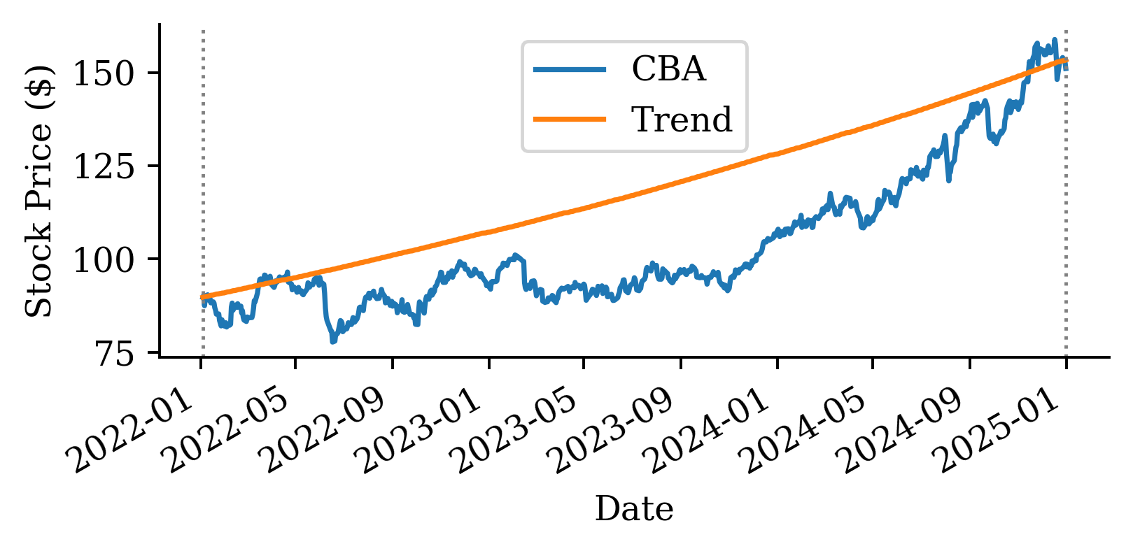
Trend fitted

# Create trend forecast for the recent period to show fitted trend
recent_trend_log = pd.Series(trend_log, index=recent_log_returns.index)
trend_start_price = get_last_price(stock, cutoff_date=recent_log_returns.index[0].strftime('%Y-%m-%d'))
recent_trend_prices = log_to_price(recent_trend_log, trend_start_price)

Code

stock.loc[recent_log_returns.index, ["CBA"]].plot(label="CBA")
recent_trend_prices.plot(label="Trend")
plt.axvline(recent_log_returns.index[0], color="gray", linestyle=":", linewidth=1)
plt.axvline(recent_log_returns.index[-1], color="gray", linestyle=":", linewidth=1)
plt.ylabel("Stock Price ($)")
plt.legend();

Trend forecasts

Code

stock.loc[start:end, ["CBA"]].plot(label="CBA")
persistence_prices.loc[start:end].plot(label="Persistence")
trend_prices.loc[start:end].plot(label="Trend")
plt.axvline("2025-01", color="black", linestyle="--")
plt.ylabel("Stock Price ($)")
plt.legend(ncol=3, loc="upper center", bbox_to_anchor=(0.5, 1.3));

Which is better?

If we look at the mean squared error (MSE) of the two models:

# Calculate MSE using the actual forecasts we computed
actual_prices = stock.loc["2025":, "CBA"]
persistence_mse = mean_squared_error(actual_prices, persistence_prices)
trend_mse = mean_squared_error(actual_prices, trend_prices)
persistence_mse, trend_mse

(254.04075100411256, 99.28717915684173)

Question

What are the units of the calculated MSE?

Answer: Since the forecasts are in $, and we square the differences, the units are in squared $.

By taking the root MSE (RMSE), the unit is back in $ which is more interpretable.

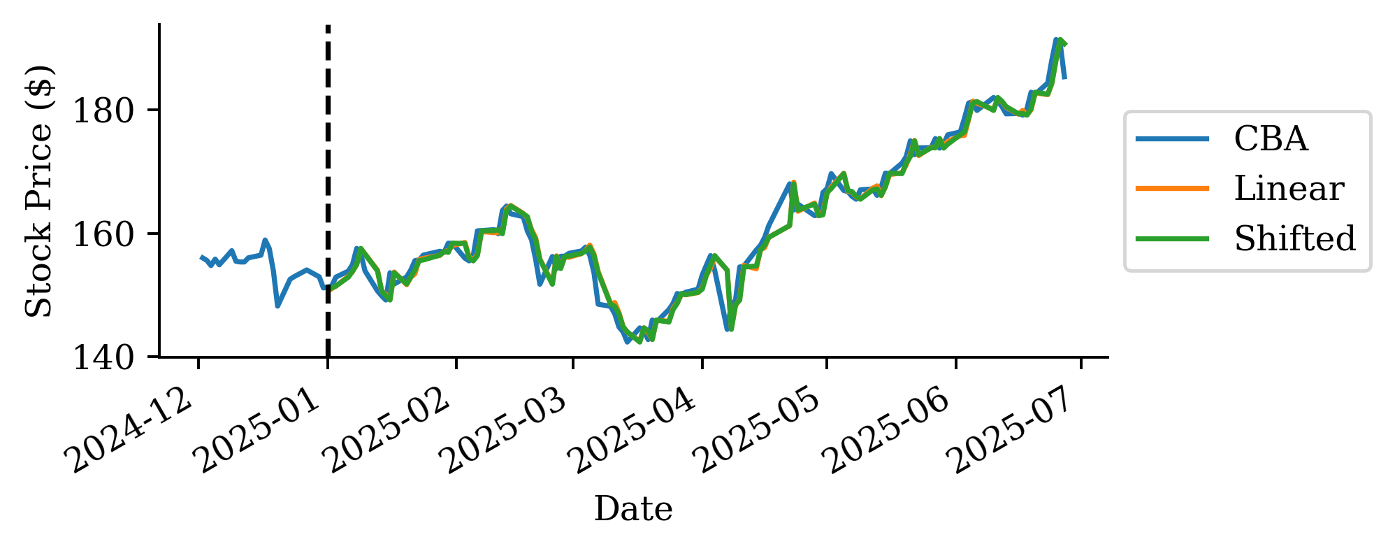
Use the history

Now let’s work with log returns instead of raw prices to create lagged features:

cba_log_shifted = stock_log["CBA"].head().shift(1)                                                  
both = pd.concat([stock_log["CBA"].head(), cba_log_shifted], axis=1, keys=["Today", "Yesterday"]) 
both

	Today	Yesterday
Date
1999-01-04	-0.010858	NaN
1999-01-05	0.000437	-0.010858
1999-01-06	0.008042	0.000437
1999-01-07	0.025859	0.008042
1999-01-08	-0.021323	0.025859

This code creates a new variable that is the log return from the previous day.

def lagged_timeseries(df, target, window=40):
    lagged = pd.DataFrame()
    for i in range(window, 0, -1):
        lagged[f"T-{i}"] = df[target].shift(i)
    lagged["T"] = df[target].values
    return lagged

This code does the same thing as above, but for 40 days, i.e. the log returns for the previous 40 days.

Lagged time series

df_lags = lagged_timeseries(stock_log, "CBA", 40)
df_lags

	T-40	T-39	T-38	T-37	T-36	T-35	T-34	T-33	T-32	T-31	...	T-9	T-8	T-7	T-6	T-5	T-4	T-3	T-2	T-1	T
Date
1999-01-04	NaN	NaN	NaN	NaN	NaN	NaN	NaN	NaN	NaN	NaN	...	NaN	NaN	NaN	NaN	NaN	NaN	NaN	NaN	NaN	-0.010858
1999-01-05	NaN	NaN	NaN	NaN	NaN	NaN	NaN	NaN	NaN	NaN	...	NaN	NaN	NaN	NaN	NaN	NaN	NaN	NaN	-0.010858	0.000437
...	...	...	...	...	...	...	...	...	...	...	...	...	...	...	...	...	...	...	...	...	...
2025-06-26	0.021968	0.003894	0.014307	-0.016222	-0.001139	-0.004689	-0.002715	0.009202	0.000838	-0.006240	...	-0.006558	0.000334	-0.001506	0.005789	0.014710	-0.001752	0.009922	0.020297	0.017232	-0.003611
2025-06-27	0.003894	0.014307	-0.016222	-0.001139	-0.004689	-0.002715	0.009202	0.000838	-0.006240	0.008153	...	0.000334	-0.001506	0.005789	0.014710	-0.001752	0.009922	0.020297	0.017232	-0.003611	-0.028454

6744 rows × 41 columns

Split into training and testing

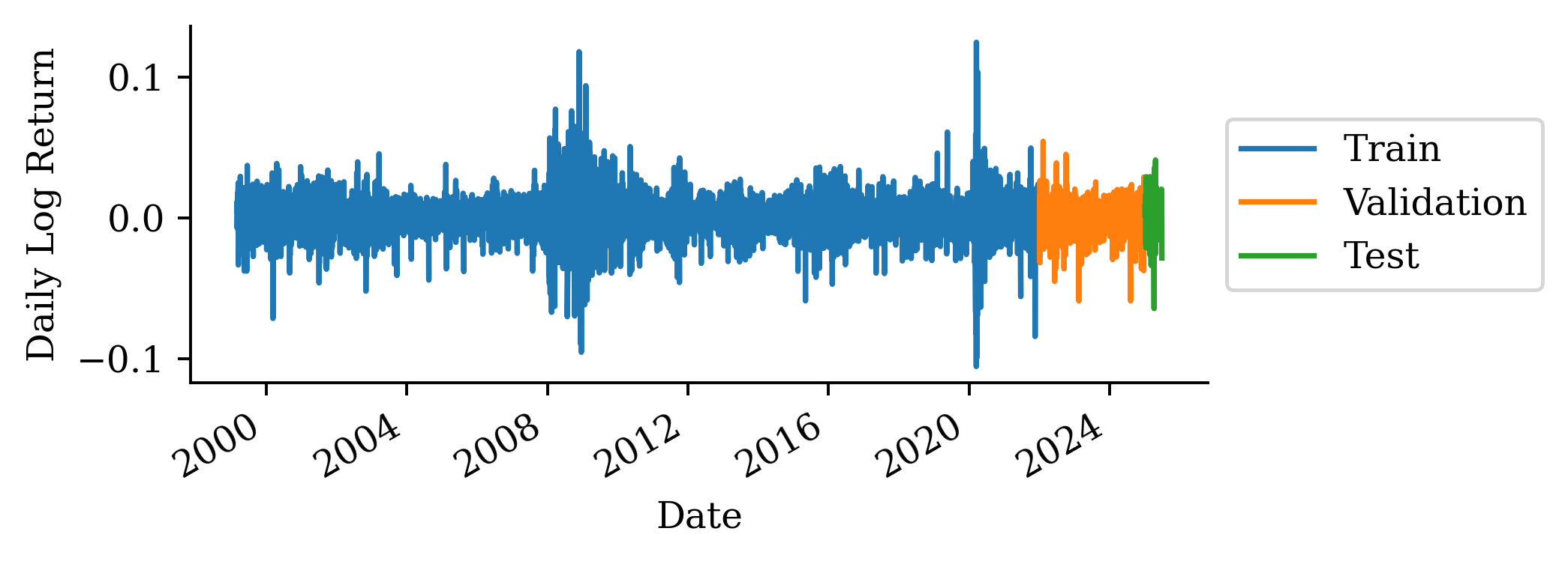
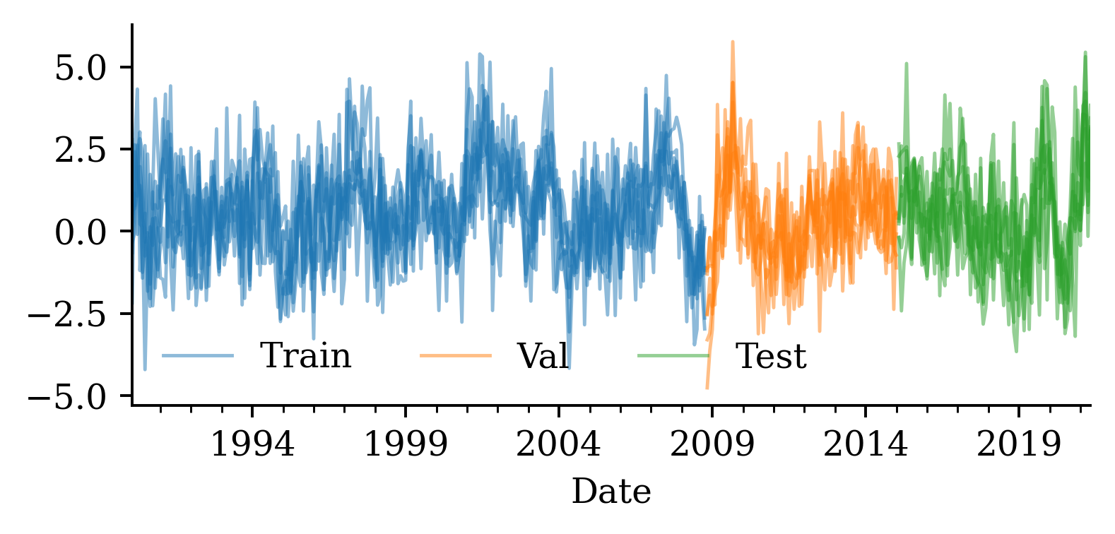
We can’t split the data randomly, as the timing of the data matters. We need to fit on older data and try to predict forward in time. Here we define:

Training data: up to 2021
Validation data: 2022-2024
Test data: 2025

# Split the data in time
X_train = df_lags.loc[:"2021"]
X_val = df_lags.loc["2022-01":"2024-12"]  # 2022-2024
X_test = df_lags.loc["2025":]  # 2025

# Remove any with NAs and split into X and y
X_train = X_train.dropna()
X_val = X_val.dropna()
X_test = X_test.dropna()

y_train = X_train.pop("T")
y_val = X_val.pop("T")
y_test = X_test.pop("T")

We want to predict today’s stock price. We need to remove today’s stock price ("T") from the features and define it as the target.

X_train.shape, y_train.shape, X_val.shape, y_val.shape, X_test.shape, y_test.shape

((5825, 40), (5825,), (757, 40), (757,), (122, 40), (122,))

Inspect the split data

X_train

	T-40	T-39	T-38	T-37	T-36	T-35	T-34	T-33	T-32	T-31	...	T-10	T-9	T-8	T-7	T-6	T-5	T-4	T-3	T-2	T-1
Date
1999-03-01	-0.010858	0.000437	0.008042	0.025859	-0.021323	-0.010573	-0.011214	-0.014823	-0.009704	0.018119	...	0.007118	-0.026875	0.000121	-0.008127	0.000000	-0.009016	0.012275	0.010156	-0.014231	-0.011912
1999-03-02	0.000437	0.008042	0.025859	-0.021323	-0.010573	-0.011214	-0.014823	-0.009704	0.018119	0.012994	...	-0.026875	0.000121	-0.008127	0.000000	-0.009016	0.012275	0.010156	-0.014231	-0.011912	0.010277
1999-03-03	0.008042	0.025859	-0.021323	-0.010573	-0.011214	-0.014823	-0.009704	0.018119	0.012994	0.010881	...	0.000121	-0.008127	0.000000	-0.009016	0.012275	0.010156	-0.014231	-0.011912	0.010277	0.004082
...	...	...	...	...	...	...	...	...	...	...	...	...	...	...	...	...	...	...	...	...	...
2021-12-29	0.015263	-0.004999	0.011656	0.013921	0.011090	0.003821	-0.012058	0.000919	-0.016106	0.008825	...	0.001327	-0.005011	-0.006273	-0.001445	0.023788	0.000807	0.003924	0.001906	0.003302	0.005181
2021-12-30	-0.004999	0.011656	0.013921	0.011090	0.003821	-0.012058	0.000919	-0.016106	0.008825	-0.001018	...	-0.005011	-0.006273	-0.001445	0.023788	0.000807	0.003924	0.001906	0.003302	0.005181	0.012541
2021-12-31	0.011656	0.013921	0.011090	0.003821	-0.012058	0.000919	-0.016106	0.008825	-0.001018	-0.003060	...	-0.006273	-0.001445	0.023788	0.000807	0.003924	0.001906	0.003302	0.005181	0.012541	0.003624

5825 rows × 40 columns

Plot the split

Code

y_train.plot()
y_val.plot()
y_test.plot()
plt.ylabel("Daily Log Return")
plt.legend(["Train", "Validation", "Test"], loc="center left", bbox_to_anchor=(1, 0.5));

Fit a linear model

lr = LinearRegression()
lr.fit(X_train, y_train);

Make a forecast for the test data:

y_pred = lr.predict(X_test)

Plot predictions in log return space

Code

log_forecasts_df = pd.DataFrame({
    "Actual": y_test,
    "Linear": y_pred
}, index=y_test.index)

log_forecasts_df.plot()
plt.ylabel("Daily Log Return")
plt.legend(loc="center left", bbox_to_anchor=(1, 0.5))

The actual log returns are far more volatile than what the linear model predicted. But let’s convert the actual and predicted returns to raw prices.

Convert to raw prices and plot

linear_log_forecasts = pd.Series(y_pred, index=y_test.index)
prev_price = stock.shift(1).loc["2025", "CBA"]
linear_price_forecasts = prev_price * np.exp(linear_log_forecasts)

Code

stock.loc[start:end, ["CBA"]].plot(label="CBA")
persistence_prices.reindex(stock.loc[start:end].index).plot(label="Persistence")
trend_prices.reindex(stock.loc[start:end].index).plot(label="Trend")
linear_price_forecasts.reindex(stock.loc[start:end].index).plot(label="Linear")
plt.axvline("2025-01", color="black", linestyle="--")
plt.ylabel("Stock Price ($)")
plt.legend(loc="center left", bbox_to_anchor=(1, 0.5));

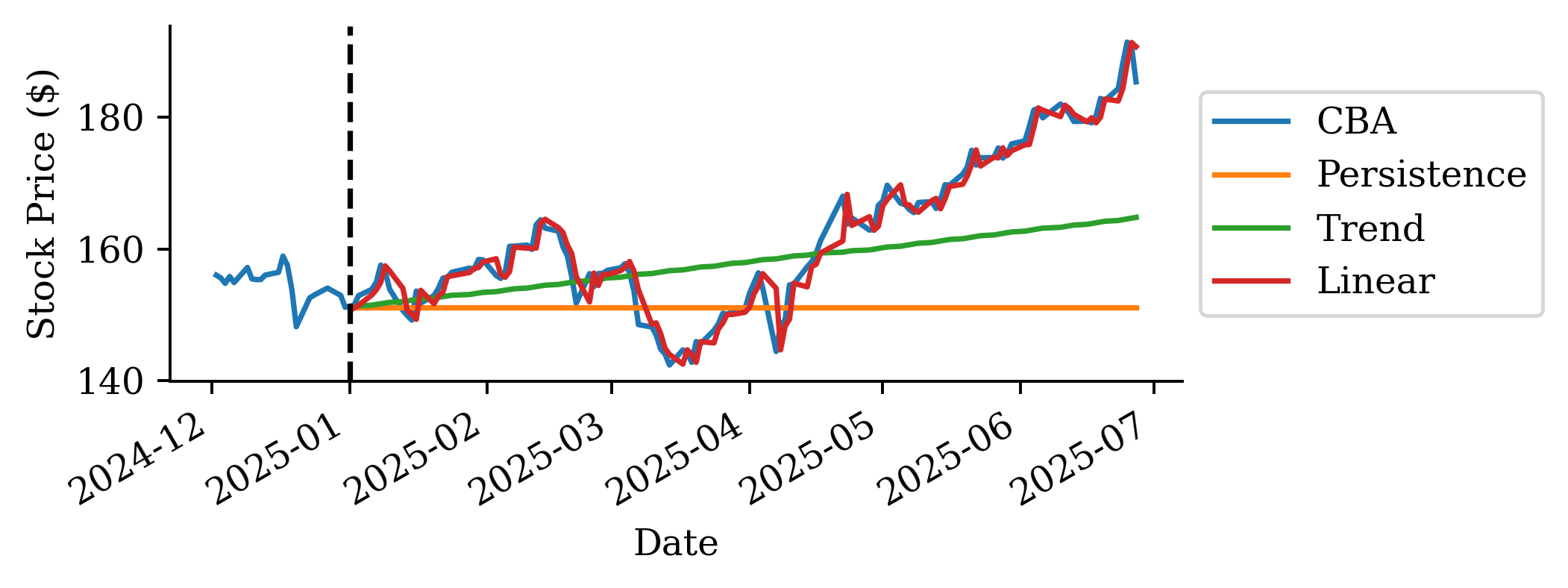
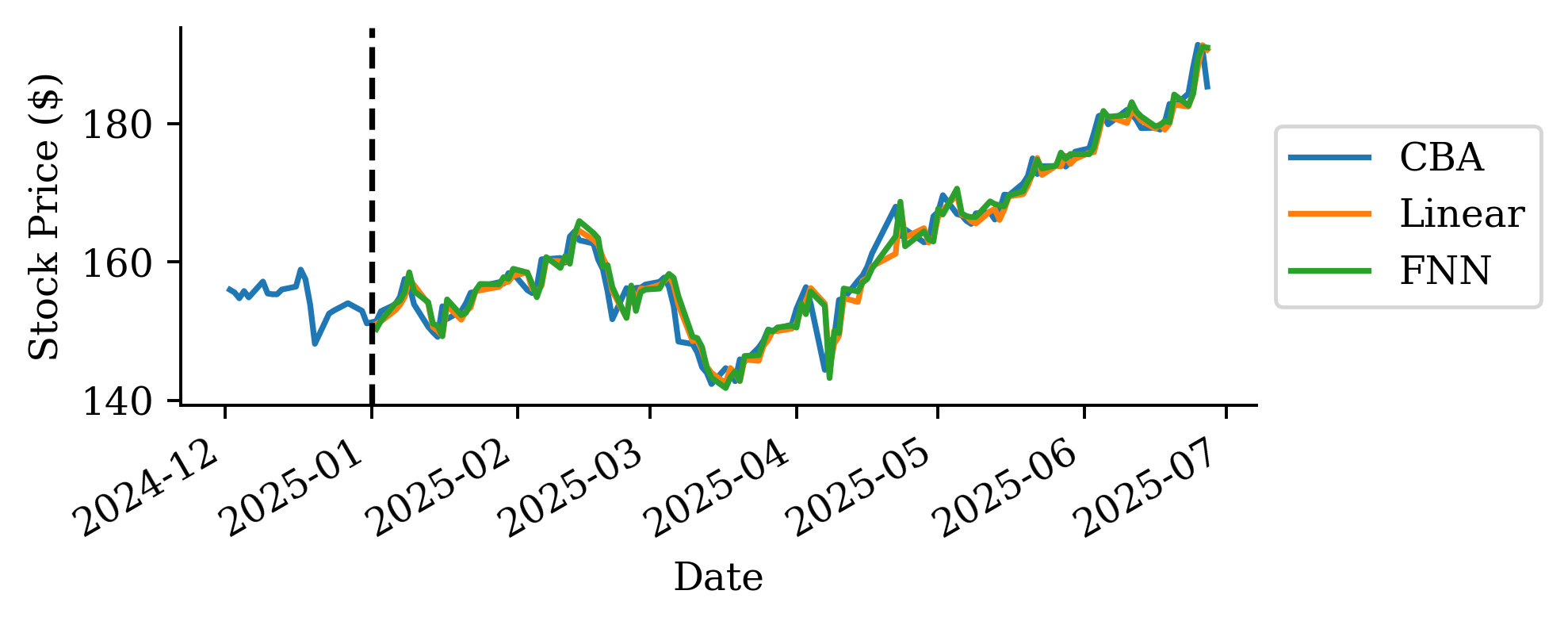
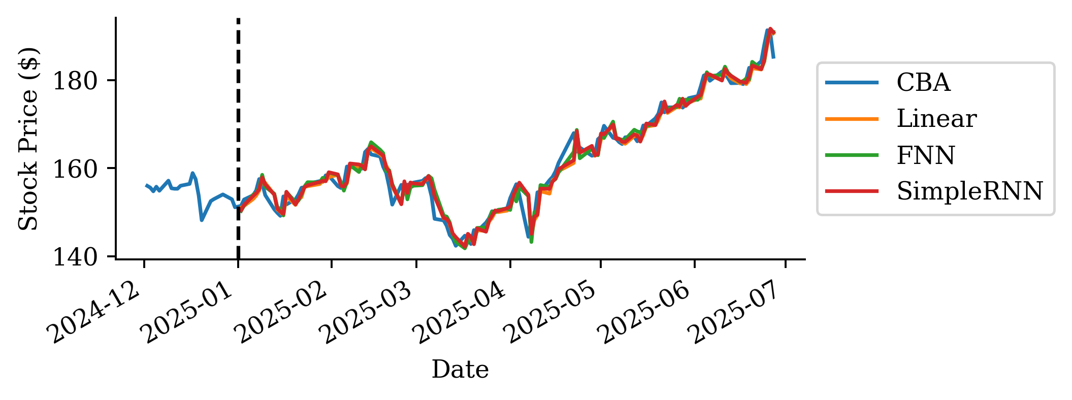
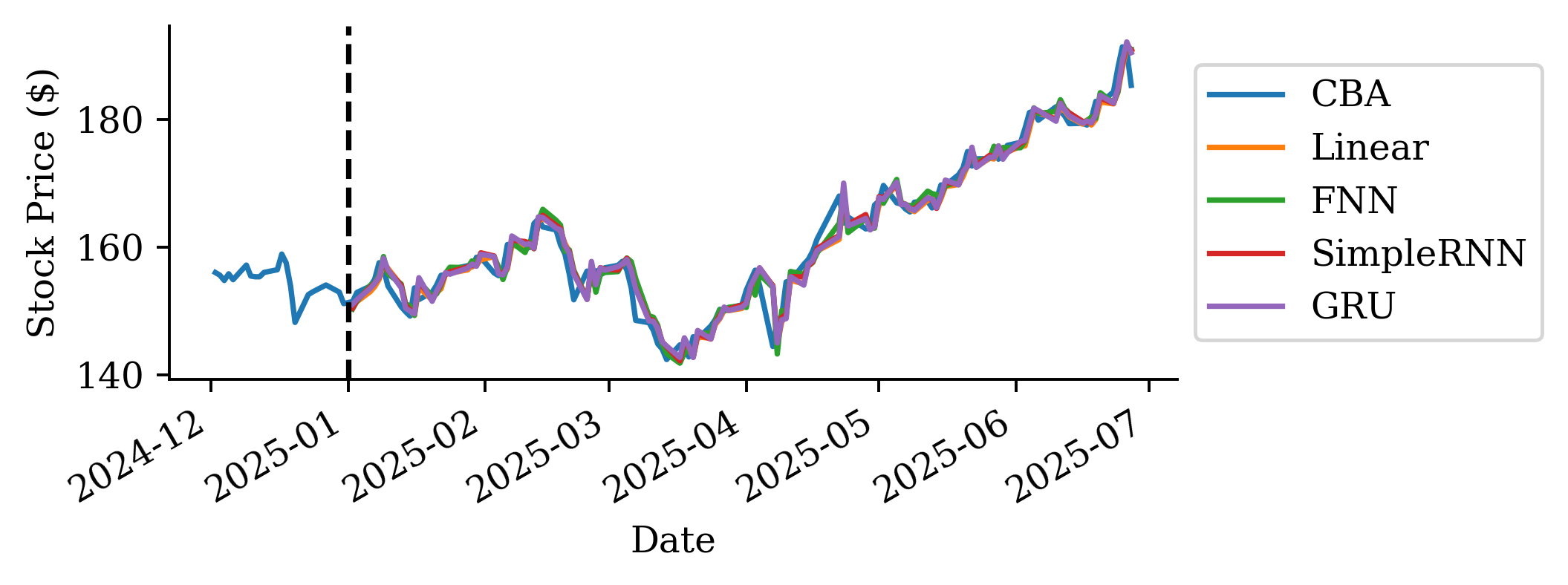
The raw prices from the linear regression are surprisingly accurate. Why is linear regression be so much better than the persistence and trend forecasts?

This is because the regression uses the last 40 days of log return data to make further predictions, unlike the persistence (assumes constant price) and trend (assume constant return) forecasts.

Distribution of log return predictions

Code

fig, (ax1, ax2) = plt.subplots(1, 2, figsize=(10, 3))

# Actual log returns
y_val.hist(bins=30, alpha=0.7, ax=ax1, label="Actual")
ax1.set_xlabel("Daily Log Return")
ax1.set_ylabel("Frequency")
ax1.set_title("Actual Log Returns")

# Predicted log returns
pd.Series(y_pred).hist(bins=30, alpha=0.7, ax=ax2, label="Predicted", color="orange")
ax2.set_xlabel("Daily Log Return")
ax2.set_ylabel("Frequency")
ax2.set_title("Predicted Log Returns")

plt.tight_layout()

The variance of the predicted log returns is much smaller than the variance of the actual log returns.

# Calculate MSE on raw prices using explicit forecast calculation
test_actual_prices = stock.loc["2025":, "CBA"]
test_linear_prices = linear_price_forecasts.loc["2025":]
linear_mse = mean_squared_error(test_actual_prices, test_linear_prices)
linear_mse

5.136664038344955

persistence_mse, trend_mse, linear_mse

(254.04075100411256, 99.28717915684173, 5.136664038344955)

Multi-step forecasts

Comparing apples to apples

The linear model is only producing one-step-ahead forecasts.

The other models are producing multi-step-ahead forecasts.

shifted_forecast = stock["CBA"].shift(1).loc["2025":]

Code

stock.loc[start:end, ["CBA"]].plot(label="CBA")
linear_price_forecasts.reindex(stock.loc[start:end].index).plot(label="Linear")
shifted_forecast.reindex(stock.loc[start:end].index).plot(label="Shifted")
plt.axvline("2025-01", color="black", linestyle="--")
plt.ylabel("Stock Price ($)")
plt.legend(loc="center left", bbox_to_anchor=(1, 0.5));

shifted_mse = mean_squared_error(stock.loc["2025":, "CBA"], shifted_forecast)
persistence_mse, trend_mse, linear_mse, shifted_mse

(254.04075100411256, 99.28717915684173, 5.136664038344955, 5.06190042634739)

In fact, the linear model is not any better than just assuming that today’s stock price will be the same as yesterday’s.

What if we want to produce multi-step-ahead linear forecasts?

Autoregressive forecasts

The linear model needs the last 90 days to make a forecast.

Idea: Make the first forecast, then use that to make the next forecast, and so on.

\begin{aligned} \hat{y}_t &= \beta_0 + \beta_1 y_{t-1} + \beta_2 y_{t-2} + \ldots + \beta_n y_{t-n} \\ \hat{y}_{t+1} &= \beta_0 + \beta_1 \hat{y}_t + \beta_2 y_{t-1} + \ldots + \beta_n y_{t-n+1} \\ \hat{y}_{t+2} &= \beta_0 + \beta_1 \hat{y}_{t+1} + \beta_2 \hat{y}_t + \ldots + \beta_n y_{t-n+2} \end{aligned} \vdots \hat{y}_{t+k} = \beta_0 + \beta_1 \hat{y}_{t+k-1} + \beta_2 \hat{y}_{t+k-2} + \ldots + \beta_n \hat{y}_{t+k-n}

Autoregressive forecasting function

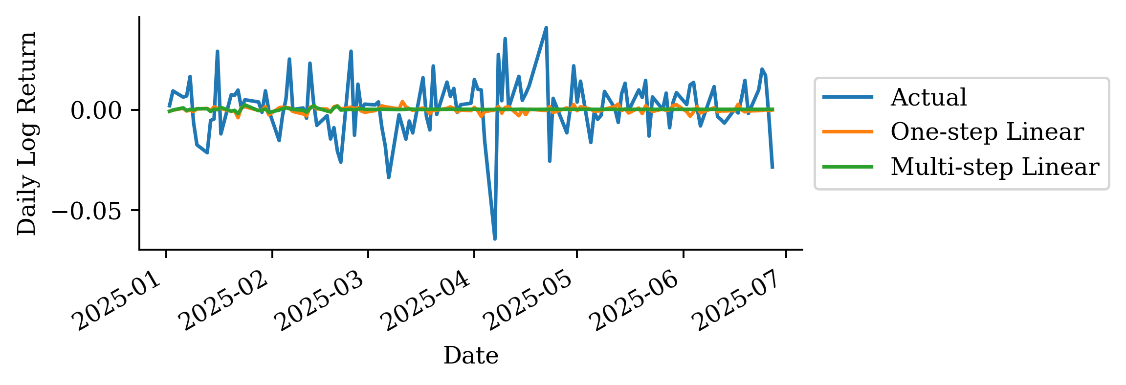
def autoregressive_forecast(model, X_val, suppress=False):
    """
    Generate a multi-step forecast using the given model.
    """
    multi_step = pd.Series(index=X_val.index, name="Multi Step")

    # Initialize the input data for forecasting
    input_data = X_val.iloc[0].values.reshape(1, -1)

    for i in range(len(multi_step)):
        # Ensure input_data has the correct feature names
        input_df = pd.DataFrame(input_data, columns=X_val.columns)
        if suppress:
            next_value = model.predict(input_df, verbose=0)
        else:
            next_value = model.predict(input_df) 

        multi_step.iloc[i] = next_value.flatten()[0]

        # Append that prediction to the input for the next forecast
        if i + 1 < len(multi_step):
            input_data = np.append(input_data[:, 1:], next_value).reshape(1, -1)

    return multi_step

Look at the autoregressive linear forecasts

lr_forecast = autoregressive_forecast(lr, X_test)
lr_multi_step_prices = log_to_price(lr_forecast, last_price)

Code

stock.loc[start:end, ["CBA"]].plot(label="CBA")
persistence_prices.reindex(stock.loc[start:end].index).plot(label="Persistence")
trend_prices.reindex(stock.loc[start:end].index).plot(label="Trend")
lr_multi_step_prices.reindex(stock.loc[start:end].index).plot(label="MS Linear")
plt.axvline("2025-01", color="black", linestyle="--")
plt.ylabel("Stock Price ($)")
plt.legend(loc="center left", bbox_to_anchor=(1, 0.5));

The multi-step-ahead linear forecast doesn’t look very good.

Compare log return forecasts

Code

log_forecasts_multistep = pd.DataFrame({
    "Actual": y_test,
    "One-step Linear": y_pred,
    "Multi-step Linear": lr_forecast
}, index=y_test.index)

log_forecasts_multistep.plot()
plt.ylabel("Daily Log Return")
plt.legend(loc="center left", bbox_to_anchor=(1, 0.5))

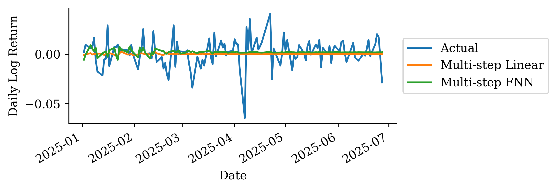
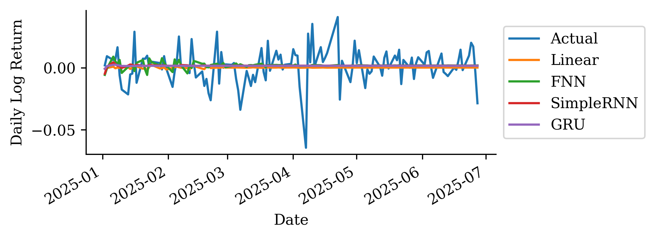
The variability in the one-step-ahead forecast is already small. The multi-step-ahead forecast reflects that and in fact the variance converges to 0 over time.

Metrics

One-step-ahead forecasts:

linear_mse, shifted_mse

(5.136664038344955, 5.06190042634739)

Multi-step-ahead forecasts:

multi_step_linear_mse = mean_squared_error(stock.loc["2025":, "CBA"], lr_multi_step_prices.loc["2025":])
persistence_mse, trend_mse, multi_step_linear_mse

(254.04075100411256, 99.28717915684173, 181.11397713761005)

We explicitly see that the mlti-step-ahead linear forecast is worse than the trend forecast.

Prefer only short windows

Code

stock.loc["2025-01":"2025-01", ["CBA"]].plot(label="CBA")
persistence_prices.loc["2025-01":"2025-01"].plot(label="Persistence")
trend_prices.loc["2025-01":"2025-01"].plot(label="Trend")
lr_multi_step_prices.loc["2025-01":"2025-01"].plot(label="MS Linear")
plt.ylabel("Stock Price ($)")
plt.legend(loc="center left", bbox_to_anchor=(1, 0.5));

It’s best not to make predictions too far in the future. There is a lot of uncertainty, and that is evident in this plot and previous plots.

“It’s tough to make predictions, especially about the future.”

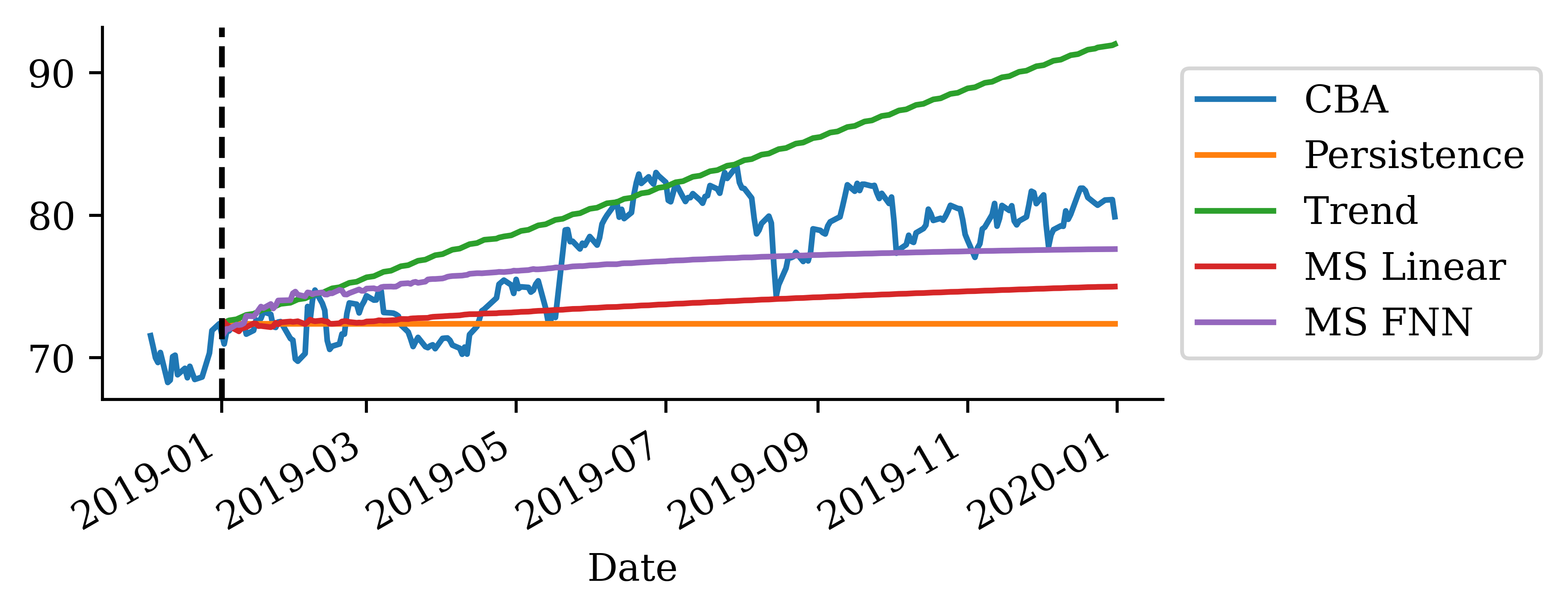
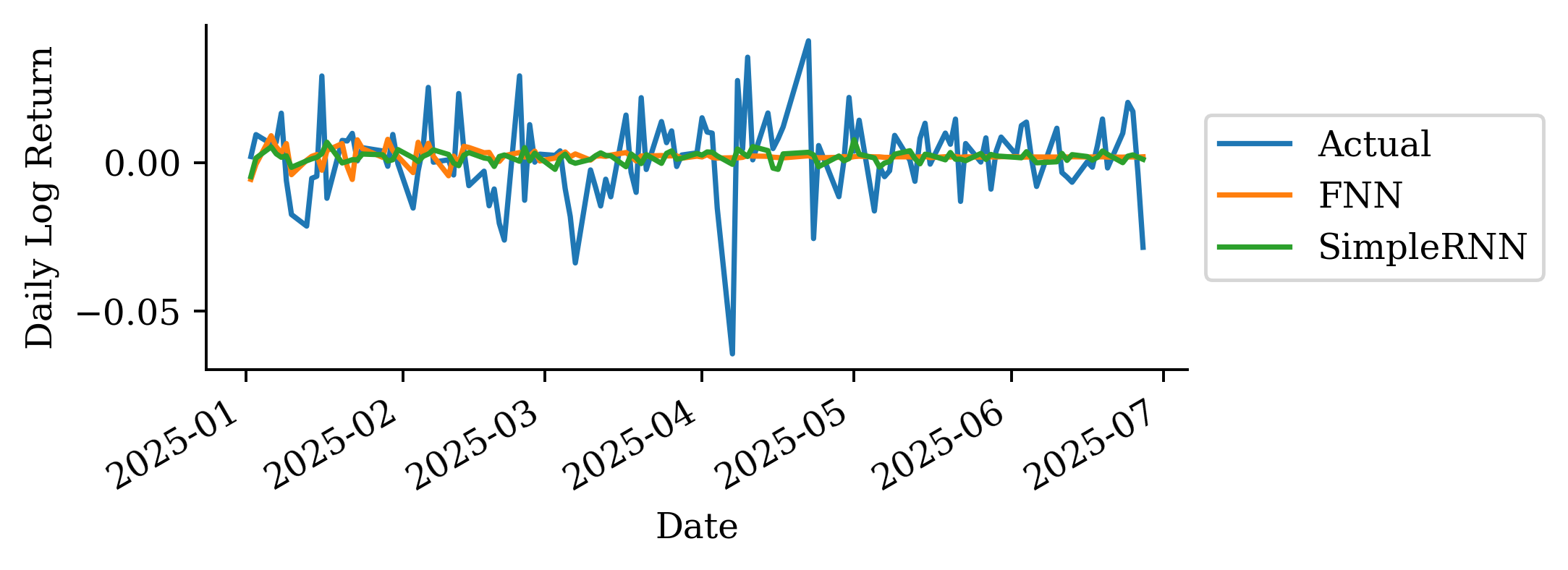
Neural network forecasts

Simple feedforward neural network

We can fit a simple feedforward NN. This is not much more complex than a linear model.

model = Sequential([
        Rescaling(1/0.02),
        Dense(32, activation="leaky_relu"),
        Dense(1)])  # Linear activation for log returns
model.compile(optimizer="adam", loss="mean_absolute_error")

The above code does the following (NN architecture): 1. Rescale the data 2. Add one hidden layer with 32 neurons 3. Final output layer is 1 neuron 4. Compile the model with selected optimizer and loss function

if Path("aus_fin_fnn_model.keras").exists():
    model = keras.models.load_model("aus_fin_fnn_model.keras")
else:
    es = EarlyStopping(patience=15, restore_best_weights=True)
    model.fit(X_train, y_train, validation_data=(X_val, y_val), epochs=500,
        callbacks=[es], verbose=0)
    model.save("aus_fin_fnn_model.keras")

model.summary()

Model: "sequential"

┏━━━━━━━━━━━━━━━━━━━━━━━━━━━━━━━━━┳━━━━━━━━━━━━━━━━━━━━━━━━┳━━━━━━━━━━━━━━━┓
┃ Layer (type)                    ┃ Output Shape           ┃       Param # ┃
┡━━━━━━━━━━━━━━━━━━━━━━━━━━━━━━━━━╇━━━━━━━━━━━━━━━━━━━━━━━━╇━━━━━━━━━━━━━━━┩
│ rescaling (Rescaling)           │ (32, 40)               │             0 │
├─────────────────────────────────┼────────────────────────┼───────────────┤
│ dense (Dense)                   │ (32, 32)               │         1,312 │
├─────────────────────────────────┼────────────────────────┼───────────────┤
│ dense_1 (Dense)                 │ (32, 1)                │            33 │
└─────────────────────────────────┴────────────────────────┴───────────────┘

 Total params: 4,037 (15.77 KB)

 Trainable params: 1,345 (5.25 KB)

 Non-trainable params: 0 (0.00 B)

 Optimizer params: 2,692 (10.52 KB)

The parameters are fitted using early stopping to minimise the mean absolute error (MAE).

Forecast and plot

y_pred = model.predict(X_test, verbose=0)

Code

# Show log return predictions
log_forecasts_nn = pd.DataFrame({
    "Actual": y_test,
    "Linear": lr.predict(X_test),
    "FNN": y_pred.flatten()
}, index=y_test.index)

log_forecasts_nn.plot()
plt.ylabel("Daily Log Return")
plt.legend(loc="center left", bbox_to_anchor=(1, 0.5))

The variance of the predicted log returns from the NN is higher; a better reflection of actual log returns.

Plot forecasts in raw price space

fnn_log_forecasts = pd.Series(y_pred.flatten(), index=y_test.index)
fnn_price_forecasts = prev_price * np.exp(fnn_log_forecasts)

Code

stock.loc[start:end, ["CBA"]].plot(label="CBA")
linear_price_forecasts.reindex(stock.loc[start:end].index).plot(label="Linear")
fnn_price_forecasts.reindex(stock.loc[start:end].index).plot(label="FNN")
plt.axvline("2025-01", color="black", linestyle="--")
plt.ylabel("Stock Price ($)")
plt.legend(loc="center left", bbox_to_anchor=(1, 0.5));

Distribution of log return predictions

Code

fig, (ax1, ax2) = plt.subplots(1, 2, figsize=(10, 3))

# Actual log returns
y_test.hist(bins=30, alpha=0.7, ax=ax1, label="Actual")
ax1.set_xlabel("Daily Log Return")
ax1.set_ylabel("Frequency")
ax1.set_title("Actual Log Returns")

# Predicted log returns
pd.Series(y_pred.flatten()).hist(bins=30, alpha=0.7, ax=ax2, label="Predicted", color="orange")
ax2.set_xlabel("Daily Log Return")
ax2.set_ylabel("Frequency")
ax2.set_title("Predicted Log Returns")

plt.tight_layout()

Autoregressive forecasts

fnn_forecast = autoregressive_forecast(model, X_test, True)
fnn_multi_step_prices = log_to_price(fnn_forecast, last_price)

Code

stock.loc[start:end, ["CBA"]].plot(label="CBA")
persistence_prices.reindex(stock.loc[start:end].index).plot(label="Persistence")
trend_prices.reindex(stock.loc[start:end].index).plot(label="Trend")
lr_multi_step_prices.reindex(stock.loc[start:end].index).plot(label="MS Linear")
fnn_multi_step_prices.reindex(stock.loc[start:end].index).plot(label="MS FNN")
plt.axvline("2025-01", color="black", linestyle="--")
plt.ylabel("Stock Price ($)")
plt.legend(loc="center left", bbox_to_anchor=(1, 0.5));

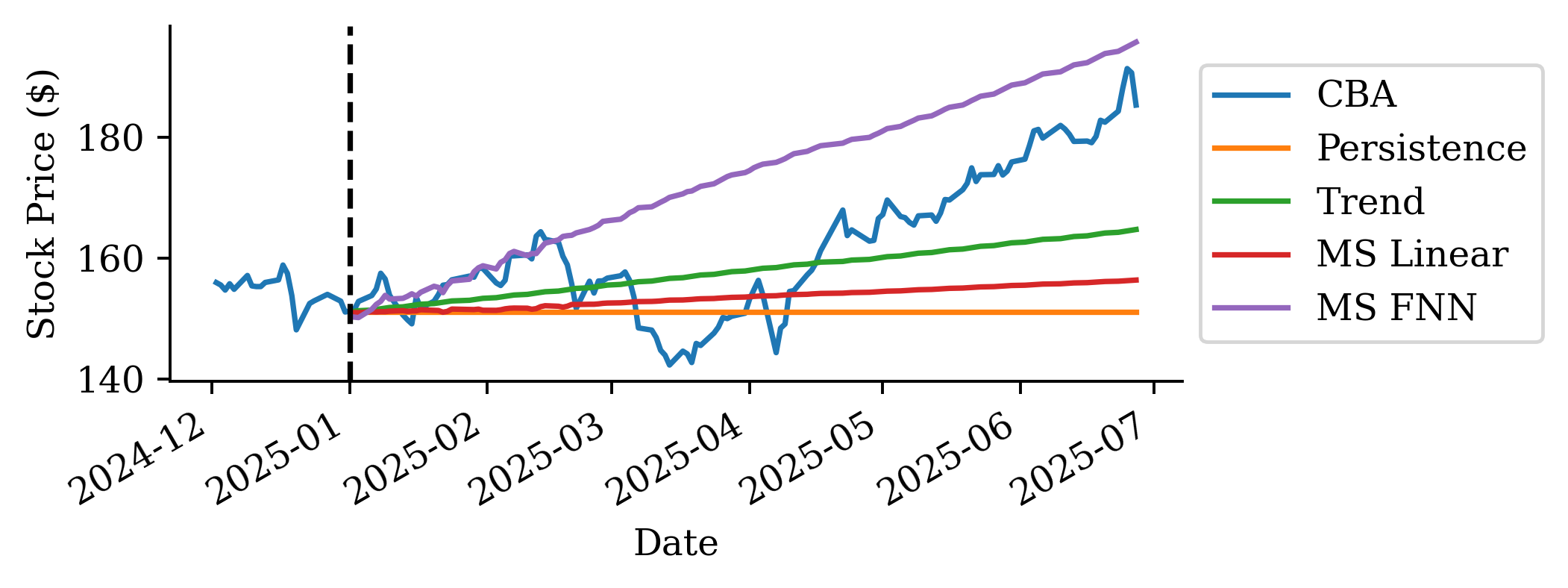
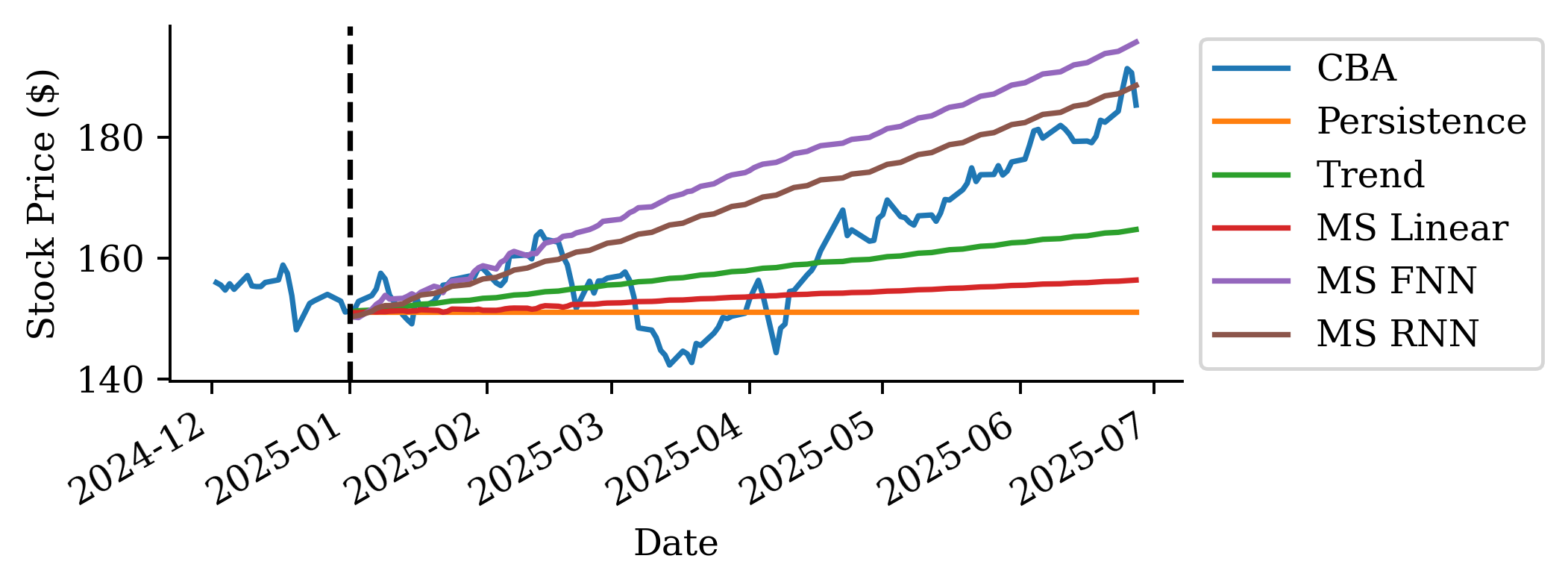
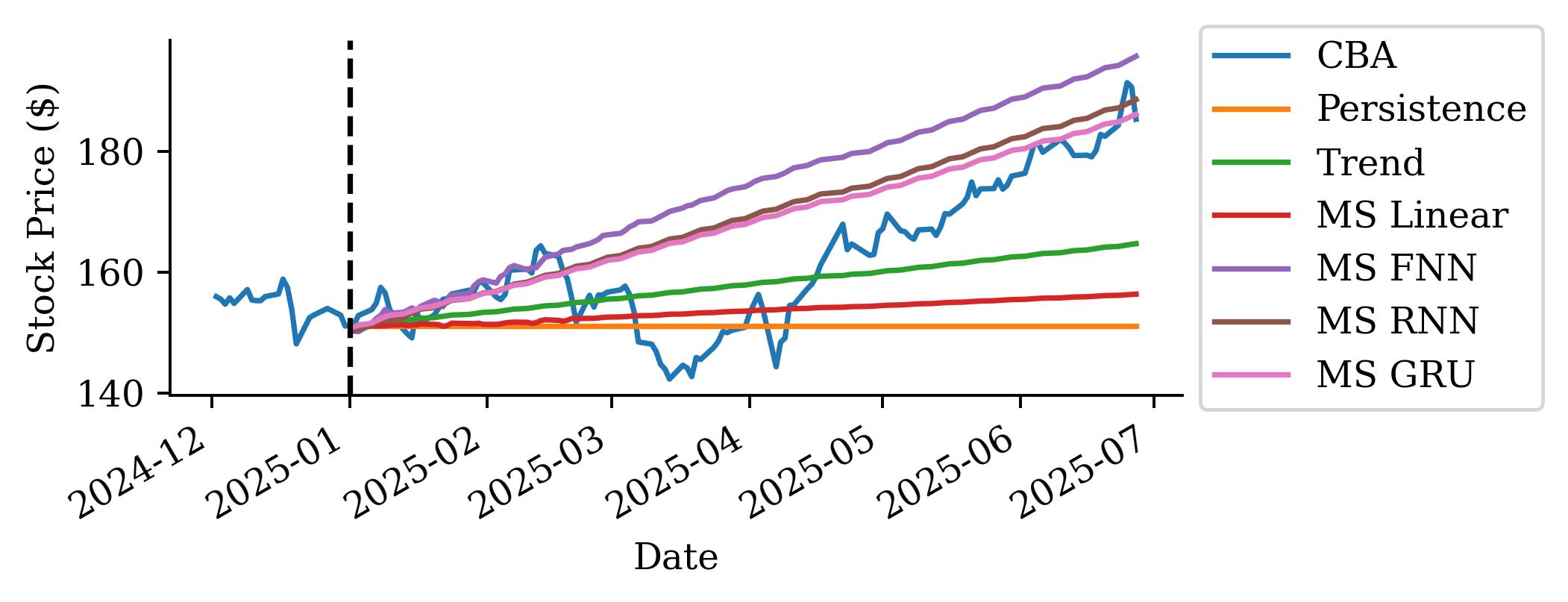
The predictions look okay for the first 2-3 months but then after that is more optimistic. Although, at the end of the forecast, the MS FNN prediction converges again to the actual price.

Compare multi-step log return forecasts

Code

log_forecasts_multistep_nn = pd.DataFrame({
    "Actual": y_test,
    "Multi-step Linear": lr_forecast,
    "Multi-step FNN": fnn_forecast
}, index=y_test.index)

log_forecasts_multistep_nn.plot()
plt.ylabel("Daily Log Return")
plt.legend(loc="center left", bbox_to_anchor=(1, 0.5));

Again, for the multi-step predictions the variance converges to 0 over time.

Metrics

One-step-ahead forecasts (MSE on raw prices):

nn_mse = mean_squared_error(stock.loc["2025":, "CBA"], fnn_price_forecasts.loc["2025":])
linear_mse, nn_mse

(5.136664038344955, 5.4393772144705546)

Multi-step-ahead forecasts (MSE on raw prices):

multi_step_fnn_mse = mean_squared_error(stock.loc["2025":, "CBA"], fnn_multi_step_prices.loc["2025":])
persistence_mse, trend_mse, multi_step_linear_mse, multi_step_fnn_mse

(254.04075100411256, 99.28717915684173, 181.11397713761005, 64.24159984960887)

Based on MSE the FNN is better than the persistence forecast but worse than the other two.

Recurrent Neural Networks

Basic facts of RNNs

A recurrent neural network is a type of neural network that is designed to process sequences of data (e.g. time series, sentences).
A recurrent neural network is any network that contains a recurrent layer.
A recurrent layer is a layer that processes data in a sequence.
An RNN can have one or more recurrent layers.
Weights are shared over time; this allows the model to be used on arbitrary-length sequences.

Applications

Forecasting: revenue forecast, weather forecast, predict disease rate from medical history, etc.
Classification: given a time series of the activities of a visitor on a website, classify whether the visitor is a bot or a human.
Event detection: given a continuous data stream, identify the occurrence of a specific event. Example: Detect utterances like “Hey Alexa” from an audio stream.
Anomaly detection: given a continuous data stream, detect anything unusual happening. Example: Detect unusual activity on the corporate network.

Origin of the name of RNNs

A recurrence relation is an equation that expresses each element of a sequence as a function of the preceding ones. More precisely, in the case where only the immediately preceding element is involved, a recurrence relation has the form

u_n = \psi(n, u_{n-1}) \quad \text{ for } \quad n > 0.

Example: Factorial n! = n (n-1)! for n > 0 given 0! = 1.

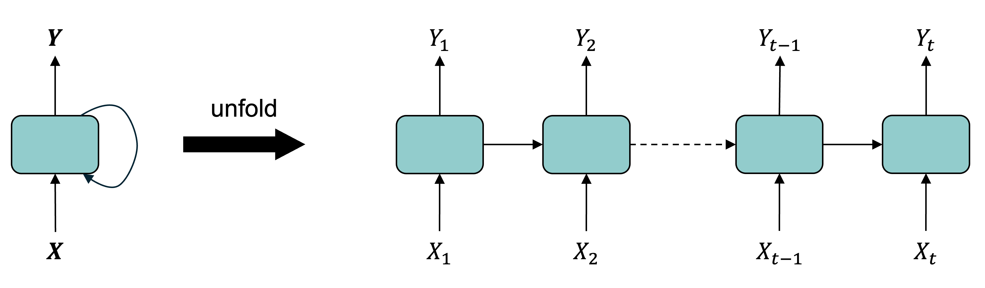
Diagram of an RNN cell

The RNN processes each data in the sequence one by one, while keeping memory of what came before.

Schematic of a recurrent neural network. E.g. SimpleRNN, LSTM, or GRU.

The RNN combines an input X_n with a processed state using inputs X_1,...,X_{n-1} to produce the output Y_n. RNNs have a cyclic information processing structure that enables them to pass information sequentially from previous inputs. RNNs can capture dependencies and patterns in sequential data, making them useful for analysing time series data.

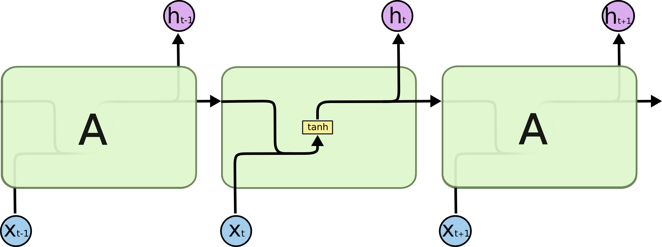
A SimpleRNN cell

All the outputs before the final one are often discarded.

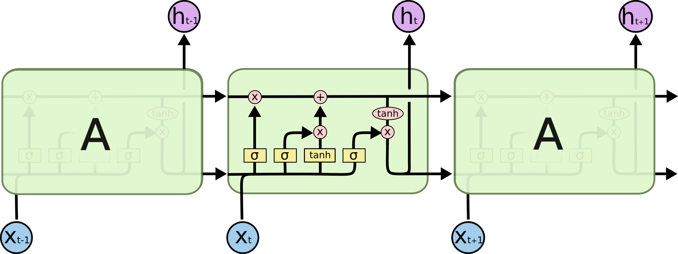
LSTM internals

Simple RNN structures encounter vanishing gradient problems, hence, struggle with learning long term dependencies. LSTM are designed to overcome this problem. LSTMs have a more complex network structure (contains more memory cells and gating mechanisms) and can better regulate the information flow.

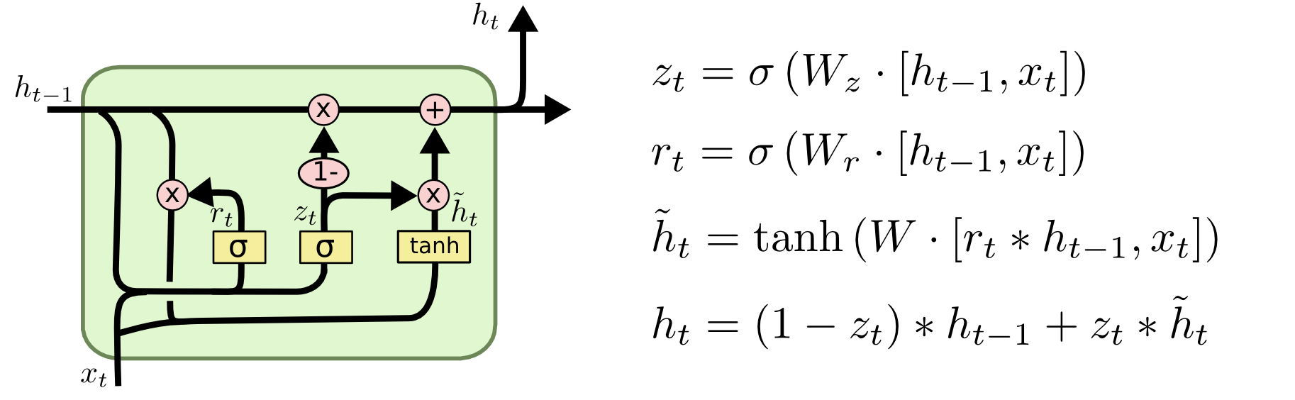
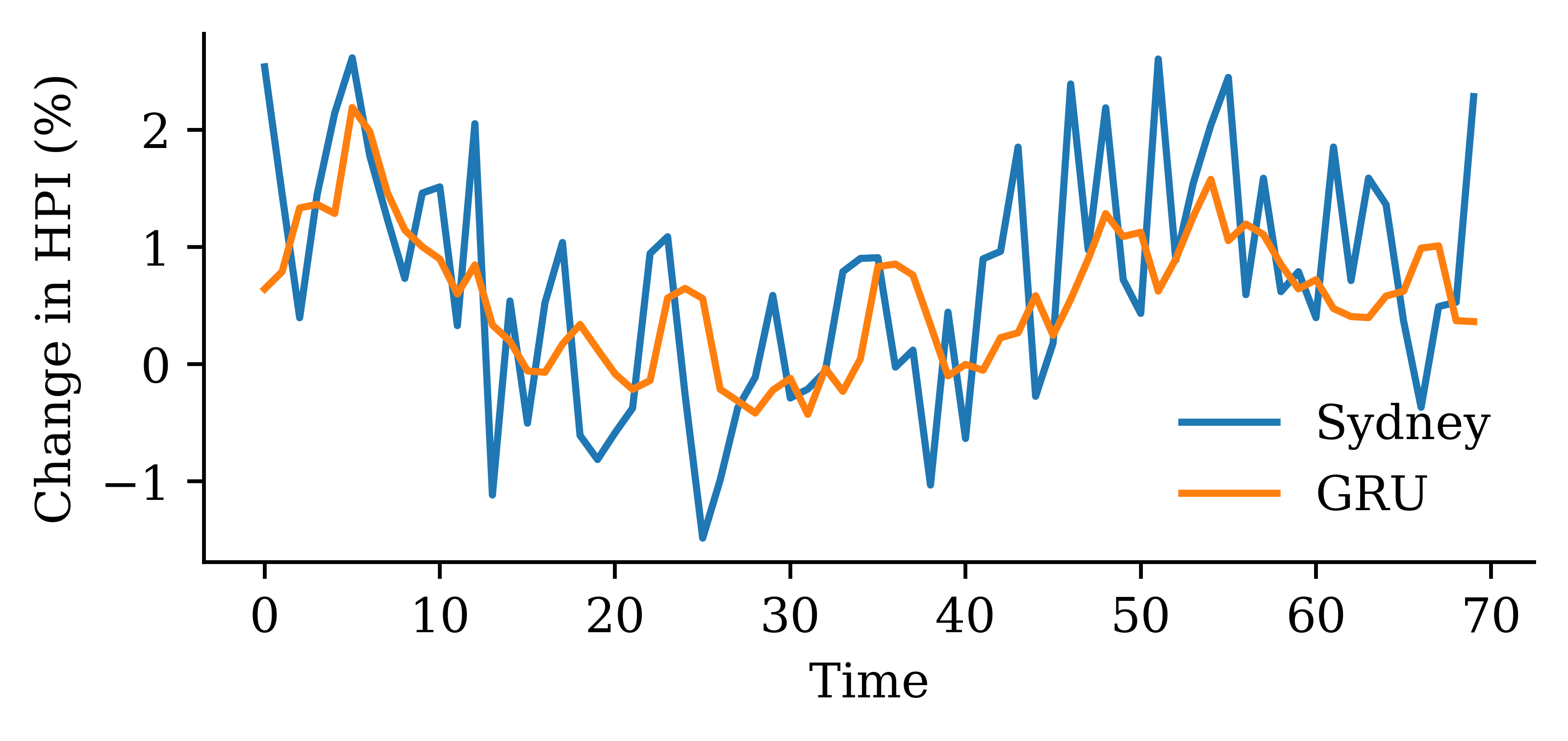
Diagram of an LSTM cell. Notation for the diagram.

GRU internals

GRUs are simpler compared to LSTM, hence, computationally more efficient than LSTMs.

Stock prediction with recurrent networks

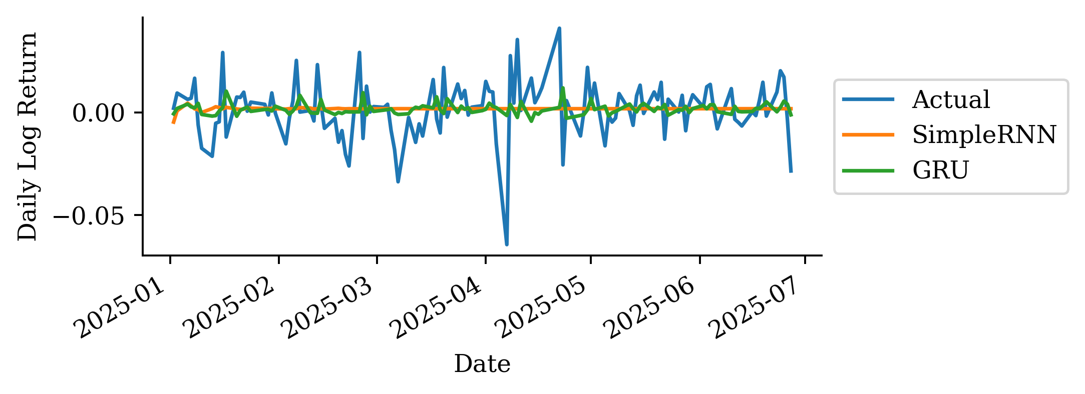
SimpleRNN

from keras.layers import SimpleRNN, Reshape
model = Sequential([
        Rescaling(1/0.02),
        Reshape((-1, 1)),
        SimpleRNN(64, activation="tanh"),
        Dense(1)])  # Linear activation for log returns
model.compile(optimizer="adam", loss="mean_absolute_error")

es = EarlyStopping(patience=15, restore_best_weights=True)
model.fit(X_train, y_train, validation_data=(X_val, y_val),
    epochs=500, callbacks=[es], verbose=0)
model.summary()

Model: "sequential_1"

┏━━━━━━━━━━━━━━━━━━━━━━━━━━━━━━━━━┳━━━━━━━━━━━━━━━━━━━━━━━━┳━━━━━━━━━━━━━━━┓
┃ Layer (type)                    ┃ Output Shape           ┃       Param # ┃
┡━━━━━━━━━━━━━━━━━━━━━━━━━━━━━━━━━╇━━━━━━━━━━━━━━━━━━━━━━━━╇━━━━━━━━━━━━━━━┩
│ rescaling_1 (Rescaling)         │ (32, 40)               │             0 │
├─────────────────────────────────┼────────────────────────┼───────────────┤
│ reshape (Reshape)               │ (32, 40, 1)            │             0 │
├─────────────────────────────────┼────────────────────────┼───────────────┤
│ simple_rnn (SimpleRNN)          │ (32, 64)               │         4,224 │
├─────────────────────────────────┼────────────────────────┼───────────────┤
│ dense_2 (Dense)                 │ (32, 1)                │            65 │
└─────────────────────────────────┴────────────────────────┴───────────────┘

 Total params: 12,869 (50.27 KB)

 Trainable params: 4,289 (16.75 KB)

 Non-trainable params: 0 (0.00 B)

 Optimizer params: 8,580 (33.52 KB)

Forecast and plot

y_pred = model.predict(X_test.to_numpy(), verbose=0)

Code

# Show log return predictions
log_forecasts_rnn = pd.DataFrame({
    "Actual": y_test,
    "FNN": fnn_forecast.values[:len(y_test)],  # Use the FNN forecast from previous section
    "SimpleRNN": y_pred.flatten()
}, index=y_test.index)

log_forecasts_rnn.plot()
plt.ylabel("Daily Log Return")
plt.legend(loc="center left", bbox_to_anchor=(1, 0.5))

Plot forecasts in raw price space

rnn_log_forecasts = pd.Series(y_pred.flatten(), index=y_test.index)
rnn_price_forecasts = prev_price * np.exp(rnn_log_forecasts)

Code

stock.loc[start:end, ["CBA"]].plot(label="CBA")
linear_price_forecasts.reindex(stock.loc[start:end].index).plot(label="Linear")
fnn_price_forecasts.reindex(stock.loc[start:end].index).plot(label="FNN")
rnn_price_forecasts.reindex(stock.loc[start:end].index).plot(label="SimpleRNN")
plt.axvline("2025-01", color="black", linestyle="--")
plt.ylabel("Stock Price ($)")
plt.legend(loc="center left", bbox_to_anchor=(1, 0.5));

Multi-step forecasts

rnn_forecast = autoregressive_forecast(model, X_test, True)
rnn_multi_step_prices = log_to_price(rnn_forecast, last_price)

Code

stock.loc[start:end, ["CBA"]].plot(label="CBA")
persistence_prices.reindex(stock.loc[start:end].index).plot(label="Persistence")
trend_prices.reindex(stock.loc[start:end].index).plot(label="Trend")
lr_multi_step_prices.reindex(stock.loc[start:end].index).plot(label="MS Linear")
fnn_multi_step_prices.reindex(stock.loc[start:end].index).plot(label="MS FNN")
rnn_multi_step_prices.reindex(stock.loc[start:end].index).plot(label="MS RNN")
plt.axvline("2025-01", color="black", linestyle="--")
plt.ylabel("Stock Price ($)")
plt.legend(loc="center left", bbox_to_anchor=(1, 0.5));

Metrics

One-step-ahead forecasts (MSE on raw prices):

rnn_mse = mean_squared_error(stock.loc["2025":, "CBA"], rnn_price_forecasts.loc["2025":])
linear_mse, nn_mse, rnn_mse

(5.136664038344955, 5.4393772144705546, 4.92958687284334)

Multi-step-ahead forecasts (MSE on raw prices):

multi_step_rnn_mse = mean_squared_error(stock.loc["2025":, "CBA"], rnn_multi_step_prices.loc["2025":])
persistence_mse, trend_mse, multi_step_linear_mse, multi_step_fnn_mse, multi_step_rnn_mse

(254.04075100411256,
 99.28717915684173,
 181.11397713761005,
 64.24159984960887,
 62.12891983723962)

Based on MSE, the RNN performs the best out of one-step forecasts, and the second best for multi-step forecasts (after the trend forecast).

GRU

The gated recurrent unit (GRU) is a type of RNN. We can select GRU in the model specification step.

from keras.layers import GRU

model = Sequential([
        Rescaling(1/0.02),
        Reshape((-1, 1)),
        GRU(16, activation="tanh"),
        Dense(1)])  # Linear activation for log returns
model.compile(optimizer="adam", loss="mean_absolute_error")

es = EarlyStopping(patience=15, restore_best_weights=True)
model.fit(X_train, y_train, validation_data=(X_val, y_val),
    epochs=500, callbacks=[es], verbose=0)
model.summary()

Model: "sequential_2"

┏━━━━━━━━━━━━━━━━━━━━━━━━━━━━━━━━━┳━━━━━━━━━━━━━━━━━━━━━━━━┳━━━━━━━━━━━━━━━┓
┃ Layer (type)                    ┃ Output Shape           ┃       Param # ┃
┡━━━━━━━━━━━━━━━━━━━━━━━━━━━━━━━━━╇━━━━━━━━━━━━━━━━━━━━━━━━╇━━━━━━━━━━━━━━━┩
│ rescaling_2 (Rescaling)         │ (32, 40)               │             0 │
├─────────────────────────────────┼────────────────────────┼───────────────┤
│ reshape_1 (Reshape)             │ (32, 40, 1)            │             0 │
├─────────────────────────────────┼────────────────────────┼───────────────┤
│ gru (GRU)                       │ (32, 16)               │           912 │
├─────────────────────────────────┼────────────────────────┼───────────────┤
│ dense_3 (Dense)                 │ (32, 1)                │            17 │
└─────────────────────────────────┴────────────────────────┴───────────────┘

 Total params: 2,789 (10.89 KB)

 Trainable params: 929 (3.63 KB)

 Non-trainable params: 0 (0.00 B)

 Optimizer params: 1,860 (7.27 KB)

Forecast and plot

y_pred = model.predict(X_test, verbose=0)

Code

# Show log return predictions
log_forecasts_gru = pd.DataFrame({
    "Actual": y_test,
    "SimpleRNN": rnn_forecast.values[:len(y_test)],  # Use the RNN forecast from previous section
    "GRU": y_pred.flatten()
}, index=y_test.index)

log_forecasts_gru.plot()
plt.ylabel("Daily Log Return")
plt.legend(loc="center left", bbox_to_anchor=(1, 0.5))

Plot forecasts in raw price space

gru_log_forecasts = pd.Series(y_pred.flatten(), index=y_test.index)
gru_price_forecasts = prev_price * np.exp(gru_log_forecasts)

Code

stock.loc[start:end, ["CBA"]].plot(label="CBA")
linear_price_forecasts.reindex(stock.loc[start:end].index).plot(label="Linear")
fnn_price_forecasts.reindex(stock.loc[start:end].index).plot(label="FNN")
rnn_price_forecasts.reindex(stock.loc[start:end].index).plot(label="SimpleRNN")
gru_price_forecasts.reindex(stock.loc[start:end].index).plot(label="GRU")
plt.axvline("2025-01", color="black", linestyle="--")
plt.ylabel("Stock Price ($)")
plt.legend(loc="center left", bbox_to_anchor=(1, 0.5));

Multi-step forecasts

gru_forecast = autoregressive_forecast(model, X_test, True)
gru_multi_step_prices = log_to_price(gru_forecast, last_price)

Code

stock.loc[start:end, ["CBA"]].plot(label="CBA")
persistence_prices.reindex(stock.loc[start:end].index).plot(label="Persistence")
trend_prices.reindex(stock.loc[start:end].index).plot(label="Trend")
lr_multi_step_prices.reindex(stock.loc[start:end].index).plot(label="MS Linear")
fnn_multi_step_prices.reindex(stock.loc[start:end].index).plot(label="MS FNN")
rnn_multi_step_prices.reindex(stock.loc[start:end].index).plot(label="MS RNN")
gru_multi_step_prices.reindex(stock.loc[start:end].index).plot(label="MS GRU")
plt.axvline("2025-01", color="black", linestyle="--")
plt.ylabel("Stock Price ($)")
plt.legend(loc="center left", bbox_to_anchor=(1, 0.5));

All multi-step log return forecasts

Code

log_forecasts_all = pd.DataFrame({
    "Actual": y_test,
    "Linear": lr_forecast,
    "FNN": fnn_forecast,
    "SimpleRNN": rnn_forecast,
    "GRU": gru_forecast
}, index=y_test.index)

log_forecasts_all.plot()
plt.ylabel("Daily Log Return")
plt.legend(loc="center left", bbox_to_anchor=(1, 0.5))

Metrics

One-step-ahead forecasts (MSE on raw prices):

gru_mse = mean_squared_error(stock.loc["2025":, "CBA"], gru_price_forecasts.loc["2025":])
linear_mse, nn_mse, rnn_mse, gru_mse

(5.136664038344955, 5.4393772144705546, 4.92958687284334, 5.133219496072287)

Multi-step-ahead forecasts (MSE on raw prices):

multi_step_gru_mse = mean_squared_error(stock.loc["2025":, "CBA"], gru_multi_step_prices.loc["2025":])
persistence_mse, trend_mse, multi_step_linear_mse, multi_step_fnn_mse, multi_step_rnn_mse, multi_step_gru_mse

(254.04075100411256,
 99.28717915684173,
 181.11397713761005,
 64.24159984960887,
 62.12891983723962,
 201.4168205668049)

Summary of all model performance

One-step forecasts

	MSE
Shifted	5.061900
Linear	5.136664
FNN	5.439377
SimpleRNN	4.929587
GRU	5.133219

Multi-step forecasts

	MSE
Persistence	254.040751
Trend	99.287179
Linear	181.113977
FNN	64.241600
SimpleRNN	62.128920
GRU	201.416821

Internals of the SimpleRNN

The rank of a time series

Say we had n observations of a time series x_1, x_2, \dots, x_n.

This \boldsymbol{x} = (x_1, \dots, x_n) would have shape (n,) & rank 1.

If instead we had a batch of b time series’

\boldsymbol{X} = \begin{pmatrix} x_7 & x_8 & \dots & x_{7+n-1} \\ x_2 & x_3 & \dots & x_{2+n-1} \\ \vdots & \vdots & \ddots & \vdots \\ x_3 & x_4 & \dots & x_{3+n-1} \\ \end{pmatrix} \,,

the batch \boldsymbol{X} would have shape (b, n) & rank 2.

Multivariate time series

Multivariate time series consists of more than 1 variable observation at a given time point. Following example has two variables x and y.

t	x	y
0	x_0	y_0
1	x_1	y_1
2	x_2	y_2
3	x_3	y_3

Say n observations of the m time series, would be a shape (n, m) matrix of rank 2.

In Keras, a batch of b of these time series has shape (b, n, m) and has rank 3.

Note

Use \boldsymbol{x}_t \in \mathbb{R}^{1 \times m} to denote the vector of all time series at time t. Here, \boldsymbol{x}_t = (x_t, y_t).

SimpleRNN

Say each prediction is a vector of size d, so \boldsymbol{y}_t \in \mathbb{R}^{1 \times d}.

Then the main equation of a SimpleRNN, given \boldsymbol{y}_0 = \boldsymbol{0}, is

\boldsymbol{y}_t = \psi\bigl( \boldsymbol{x}_t \boldsymbol{W}_x + \boldsymbol{y}_{t-1} \boldsymbol{W}_y + \boldsymbol{b} \bigr) .

Here, \begin{aligned} &\boldsymbol{x}_t \in \mathbb{R}^{1 \times m}, \boldsymbol{W}_x \in \mathbb{R}^{m \times d}, \\ &\boldsymbol{y}_{t-1} \in \mathbb{R}^{1 \times d}, \boldsymbol{W}_y \in \mathbb{R}^{d \times d}, \text{ and } \boldsymbol{b} \in \mathbb{R}^{d}. \end{aligned}

At each time step, a simple Recurrent Neural Network (RNN) takes an input vector x_t, incorporates it with the information from the previous hidden state {y}_{t-1} and produces an output vector at each time step y_t. The hidden state helps the network remember the context of the previous inputs and states, enabling it to make informed predictions about what comes next in the sequence. In a simple RNN, the output at time (t-1) is the same as the hidden state at time t.

SimpleRNN (in batches)

The difference between RNN and RNNs with batch processing lies in the way how the neural network handles sequences of input data. With batch processing, the model processes multiple (b) input sequences simultaneously. The training data is grouped into batches, and the weights are updated based on the average error across the entire batch. Batch processing often results in more stable weight updates, as the model learns from a diverse set of examples in each batch, reducing the impact of noise in individual sequences.

Say we operate on batches of size b, then \boldsymbol{Y}_t \in \mathbb{R}^{b \times d}.

The main equation of a SimpleRNN, given \boldsymbol{Y}_0 = \boldsymbol{0}, is \boldsymbol{Y}_t = \psi\bigl( \boldsymbol{X}_t \boldsymbol{W}_x + \boldsymbol{Y}_{t-1} \boldsymbol{W}_y + \boldsymbol{b} \bigr) . Here, \begin{aligned} &\boldsymbol{X}_t \in \mathbb{R}^{b \times m}, \boldsymbol{W}_x \in \mathbb{R}^{m \times d}, \\ &\boldsymbol{Y}_{t-1} \in \mathbb{R}^{b \times d}, \boldsymbol{W}_y \in \mathbb{R}^{d \times d}, \text{ and } \boldsymbol{b} \in \mathbb{R}^{d}. \end{aligned}

Simple Keras demo

1num_obs = 4
2num_time_steps = 3
3num_time_series = 2

X = (
    np.arange(num_obs * num_time_steps * num_time_series)
    .astype(np.float32)
    .reshape([num_obs, num_time_steps, num_time_series])
4)

output_size = 1
y = np.array([0, 0, 1, 1])

1: Defines the number of observations
2: Defines the number of time steps
3: Defines the number of time series
4: Reshapes the array to a range 3 tensor (4,3,2)

1X[:2]

1: Selects the first two slices along the first dimension. Since the tensor of dimensions (4,3,2), X[:2] selects the first two slices (0 and 1) along the first dimension, and returns a sub-tensor of shape (2,3,2).

array([[[ 0.,  1.],
        [ 2.,  3.],
        [ 4.,  5.]],

       [[ 6.,  7.],
        [ 8.,  9.],
        [10., 11.]]], dtype=float32)

1X[2:]

1: Selects the last two slices along the first dimension. The first dimension (axis=0) has size 4. Therefore, X[2:] selects the last two slices (2 and 3) along the first dimension, and returns a sub-tensor of shape (2,3,2).

array([[[12., 13.],
        [14., 15.],
        [16., 17.]],

       [[18., 19.],
        [20., 21.],
        [22., 23.]]], dtype=float32)

Keras’ SimpleRNN

As usual, the SimpleRNN is just a layer in Keras.

1from keras.layers import SimpleRNN

2random.seed(1234)
3model = Sequential([SimpleRNN(output_size, activation="sigmoid")])
4model.compile(loss="binary_crossentropy", metrics=["accuracy"])

5hist = model.fit(X, y, epochs=500, verbose=False)
6model.evaluate(X, y, verbose=False)

1: Imports the SimpleRNN layer from the Keras library
2: Sets the seed for the random number generator to ensure reproducibility
3: Defines a simple RNN with one output node and sigmoid activation function
4: Specifies binary crossentropy as the loss function (usually used in classification problems), and specifies “accuracy” as the metric to be monitored during training
5: Trains the model for 500 epochs and saves output as hist
6: Evaluates the model to obtain a value for the loss and accuracy

[8.05906867980957, 0.5]

The predicted probabilities on the training set are:

model.predict(X, verbose=0)

array([[8.56e-05],
       [2.25e-10],
       [5.98e-16],
       [1.59e-21]], dtype=float32)

SimpleRNN weights

To verify the results of predicted probabilities, we can obtain the weights of the fitted model and calculate the outcome manually as follows.

model.get_weights()

[array([[-1.47],
        [-0.67]], dtype=float32),
 array([[0.99]], dtype=float32),
 array([-0.14], dtype=float32)]

def sigmoid(x):
    return 1 / (1 + np.exp(-x))


W_x, W_y, b = model.get_weights()

Y = np.zeros((num_obs, output_size), dtype=np.float32)
for t in range(num_time_steps):
    X_t = X[:, t, :]
    z = X_t @ W_x + Y @ W_y + b
    Y = sigmoid(z)

Y

array([[8.56e-05],
       [2.25e-10],
       [5.98e-16],
       [1.59e-21]], dtype=float32)

Other recurrent network variants

Input and output sequences

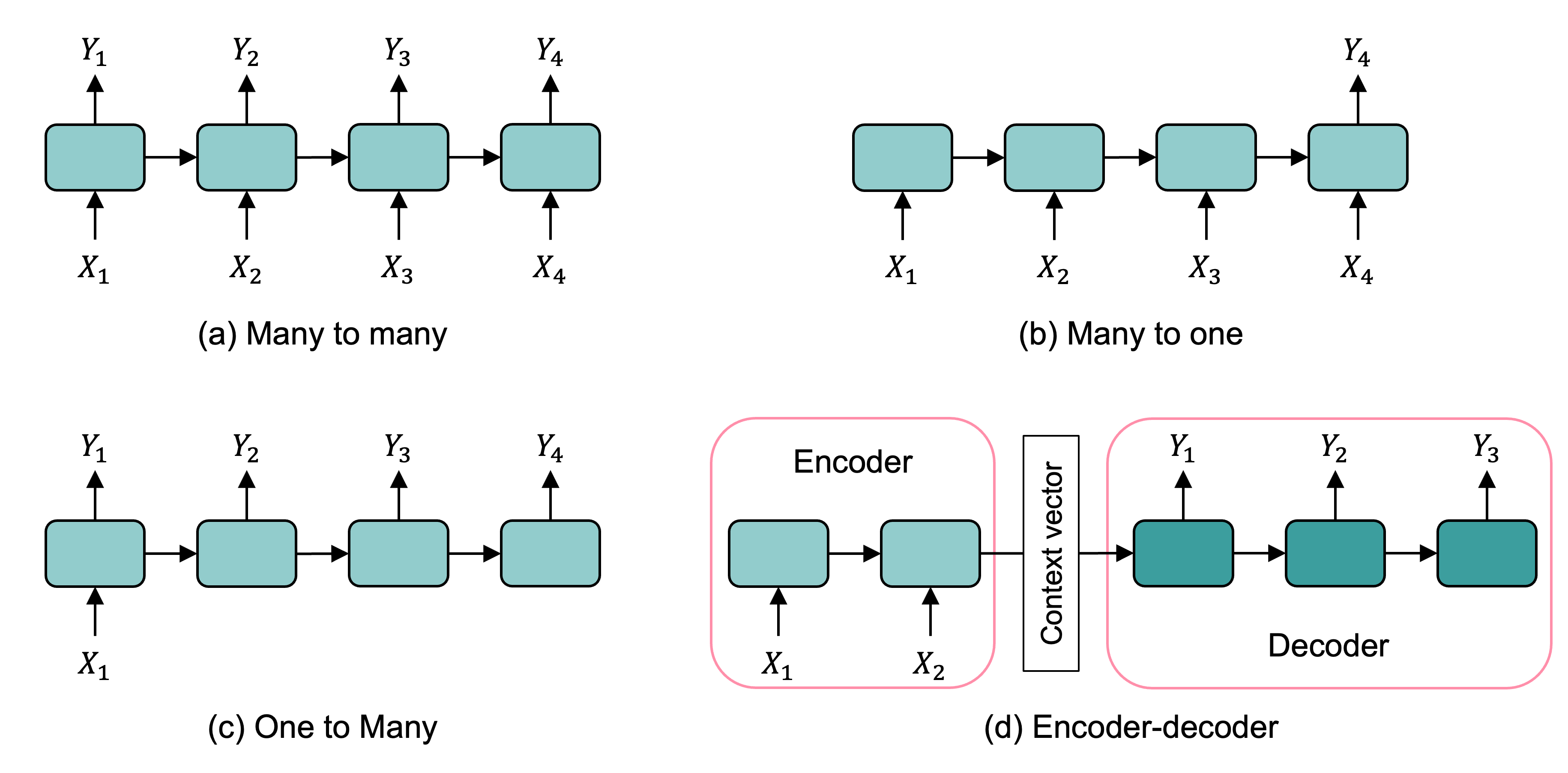
Categories of recurrent neural networks: sequence to sequence, sequence to vector, vector to sequence, encoder-decoder network.

Input and output sequences

Sequence to sequence: Useful for predicting time series such as using prices over the last N days to output the prices shifted one day into the future (i.e. from N-1 days ago to tomorrow.)
Sequence to vector: ignore all outputs in the previous time steps except for the last one. Example: give a sentiment score to a sequence of words corresponding to a movie review.

Input and output sequences

Vector to sequence: feed the network the same input vector over and over at each time step and let it output a sequence. Example: given that the input is an image, find a caption for it. The image is treated as an input vector (pixels in an image do not follow a sequence). The caption is a sequence of textual description of the image. A dataset containing images and their descriptions is the input of the RNN.
The Encoder-Decoder: The encoder is a sequence-to-vector network. The decoder is a vector-to-sequence network. Example: Feed the network a sequence in one language. Use the encoder to convert the sentence into a single vector representation. The decoder decodes this vector into the translation of the sentence in another language.

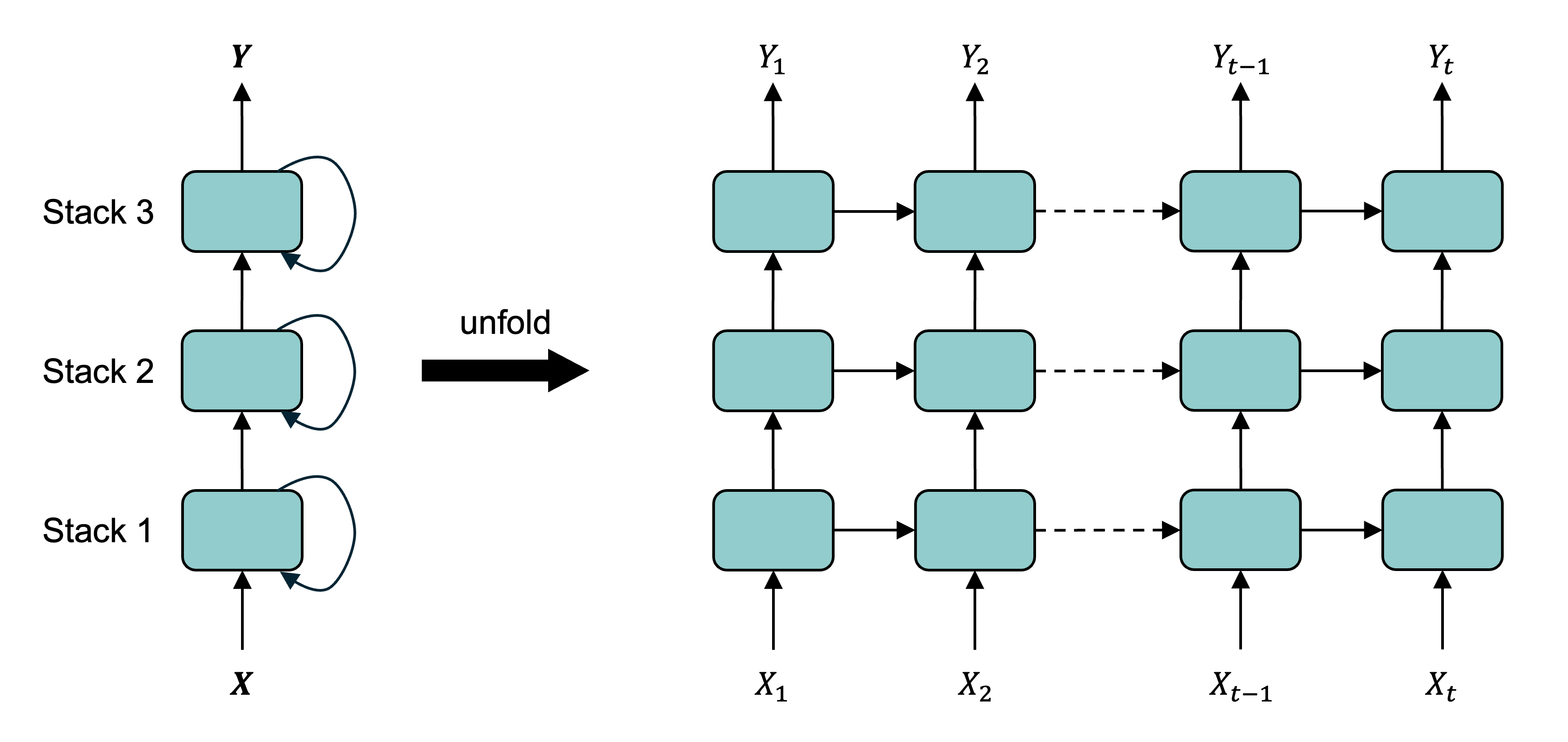
Recurrent layers can be stacked.

The output from a hidden state can be used as input for another hidden layer of RNN processing. This is called stacking, or a stacked RNN.

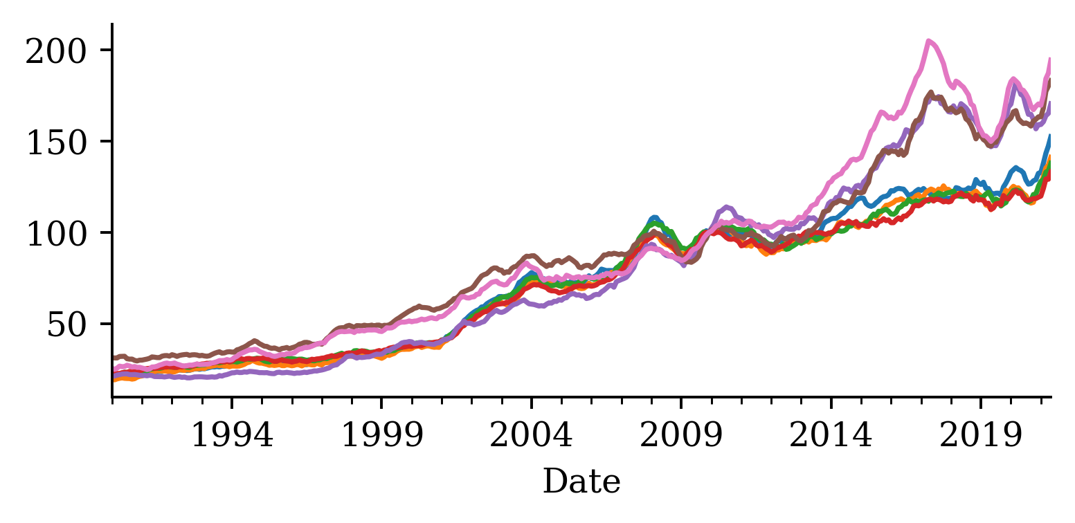
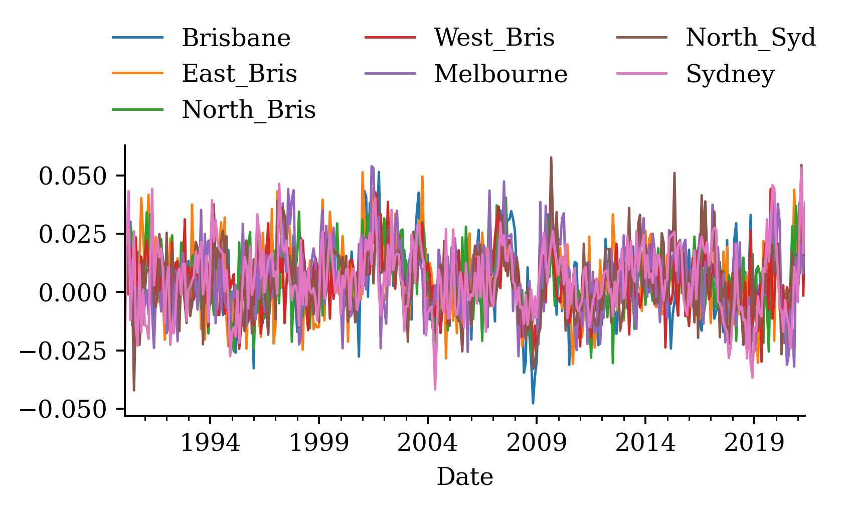
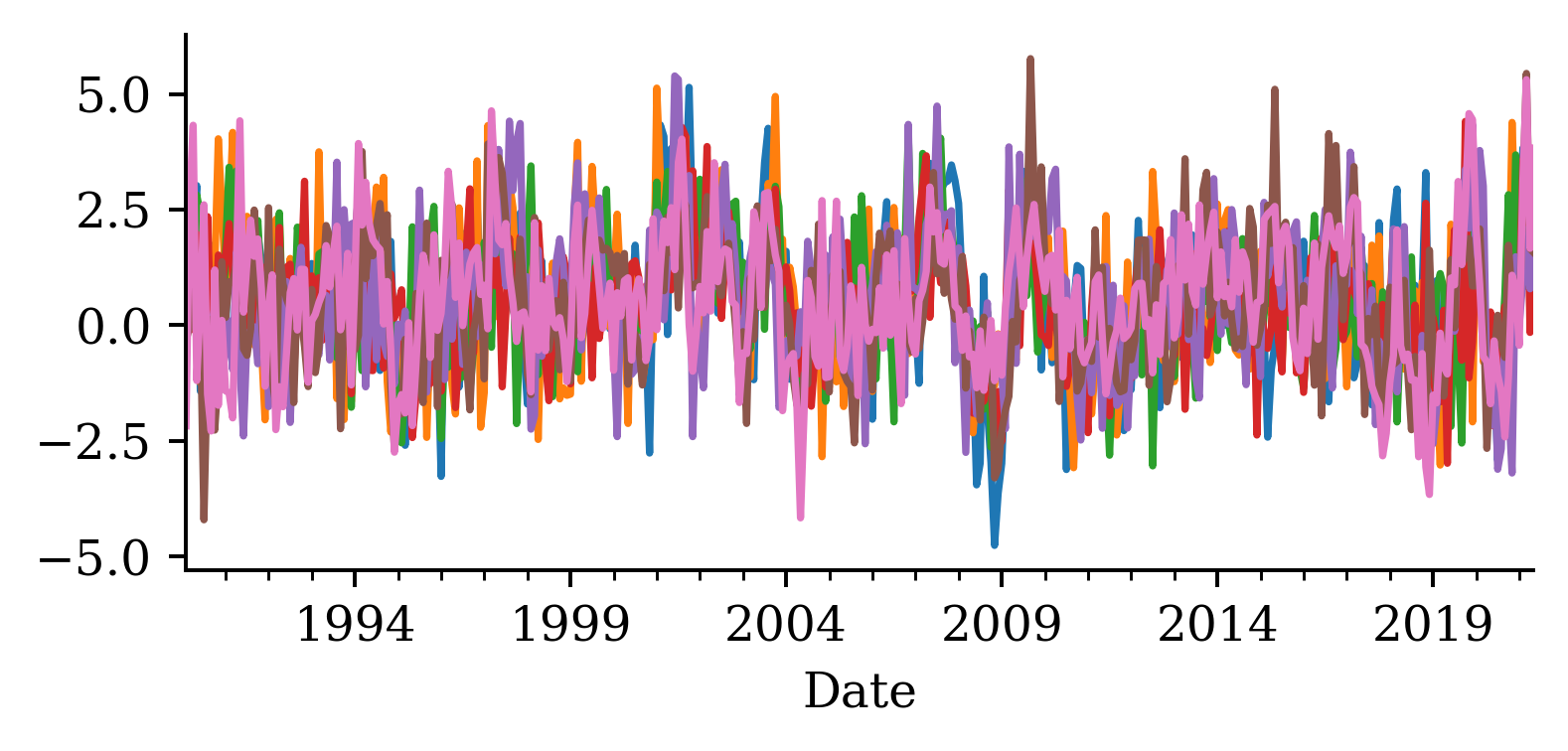
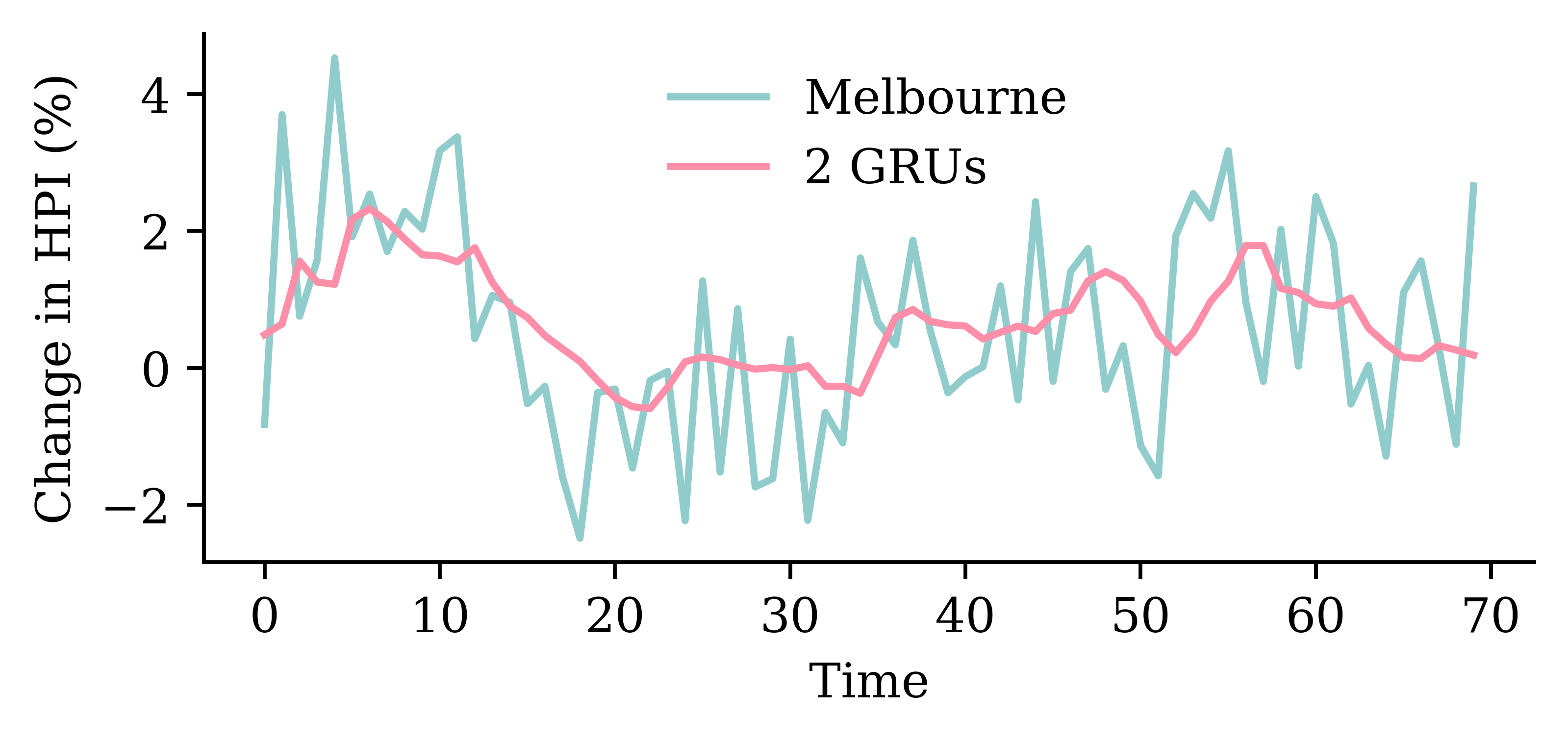
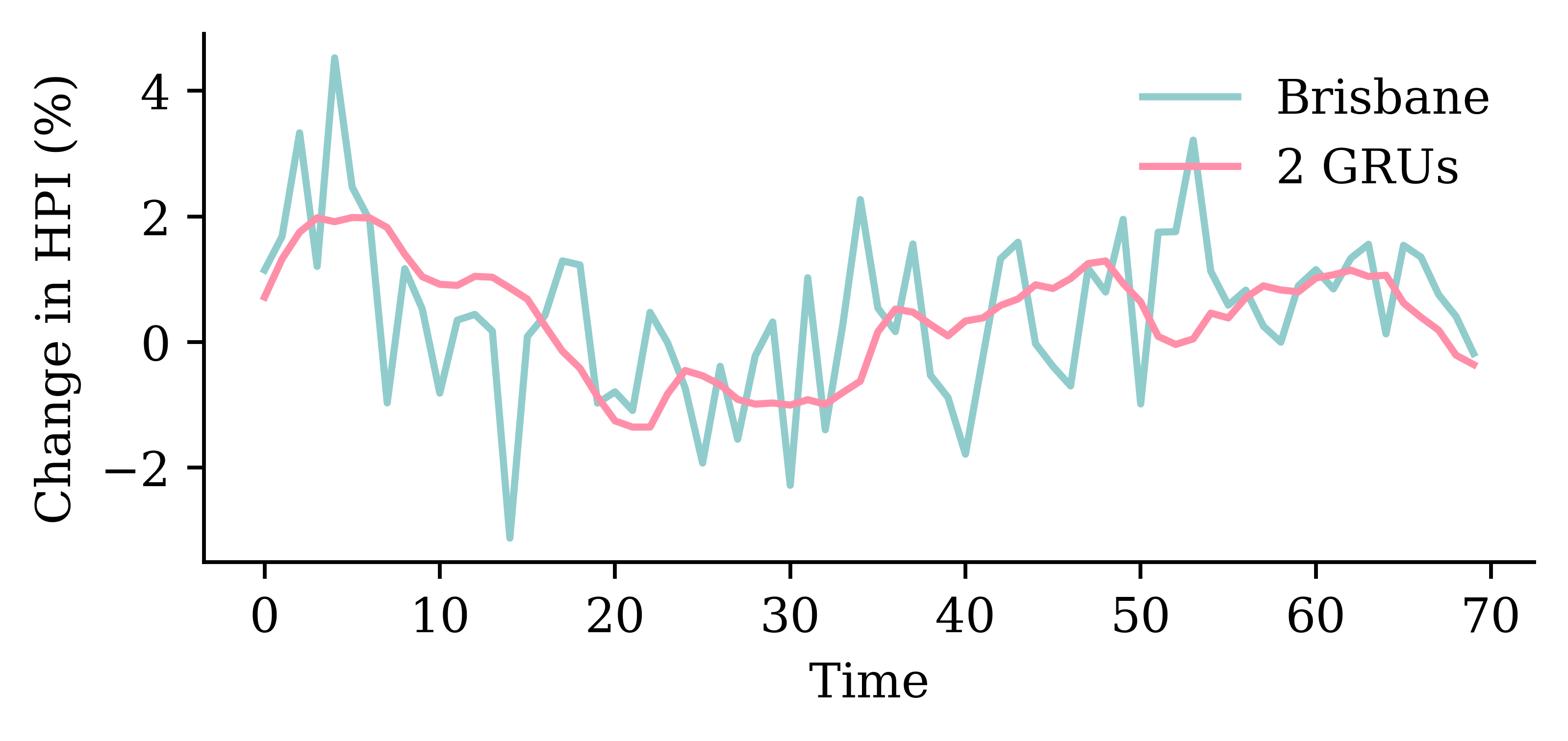
CoreLogic Hedonic Home Value Index

Australian House Price Indices

Note

I apologise in advance for not being able to share this dataset with anyone (it is not mine to share).

Percentage changes

changes = house_prices.pct_change().dropna()
changes.round(2)

	Brisbane	East_Bris	North_Bris	West_Bris	Melbourne	North_Syd	Sydney
Date
1990-02-28	0.03	-0.01	0.01	0.01	0.00	-0.00	-0.02
1990-03-31	0.01	0.03	0.01	0.01	0.02	-0.00	0.03
1990-04-30	0.02	0.02	0.01	-0.00	0.01	0.03	0.04
...	...	...	...	...	...	...	...
2021-03-31	0.04	0.04	0.03	0.04	0.02	0.05	0.05
2021-04-30	0.03	0.01	0.01	-0.00	0.01	0.02	0.02
2021-05-31	0.03	0.03	0.03	0.03	0.03	0.02	0.04

376 rows × 7 columns

Percentage changes

changes.plot();

The size of the changes

changes.mean()

Brisbane      0.005496
East_Bris     0.005416
North_Bris    0.005024
West_Bris     0.004842
Melbourne     0.005677
North_Syd     0.004819
Sydney        0.005526
dtype: float64

changes *= 100

changes.mean()

Brisbane      0.549605
East_Bris     0.541562
North_Bris    0.502390
West_Bris     0.484204
Melbourne     0.567700
North_Syd     0.481863
Sydney        0.552641
dtype: float64

changes.plot(legend=False);

Split without shuffling

num_train = int(0.6 * len(changes))
num_val = int(0.2 * len(changes))
num_test = len(changes) - num_train - num_val
print(f"# Train: {num_train}, # Val: {num_val}, # Test: {num_test}")

# Train: 225, # Val: 75, # Test: 76

Subsequences of a time series

We can use numpy to convert a time series into subsequences/chunks using a sliding window.

integers = np.arange(10)
seq_len = 3

X = np.stack([integers[i : i + seq_len] for i in range(len(integers) - seq_len)])
y = integers[seq_len:]

for i in range(len(X)):
    print(X[i].tolist(), int(y[i]))

[0, 1, 2] 3
[1, 2, 3] 4
[2, 3, 4] 5
[3, 4, 5] 6
[4, 5, 6] 7
[5, 6, 7] 8
[6, 7, 8] 9

Predicting Sydney House Prices

Creating input arrays

def make_sequences(data, targets, seq_len, start_index=0, end_index=None):
    data = np.asarray(data, dtype=np.float32)
    targets = np.asarray(targets, dtype=np.float32)
    if end_index is None:
        end_index = len(data)
    n = end_index - start_index - seq_len + 1
    X = np.stack([data[start_index + i : start_index + i + seq_len] for i in range(n)])
    y = targets[start_index : start_index + n]
    return X, y

# Num. of input time series.
num_ts = changes.shape[1]

# How many prev. months to use.
seq_length = 6

# Predict the next month ahead.
ahead = 1

# The index of the first target.
delay = seq_length + ahead - 1

# Which suburb to predict.
target_suburb = changes["Sydney"]

X_train, y_train = make_sequences(
    changes[:-delay], target_suburb[delay:],
    seq_length, end_index=num_train,
)

X_val, y_val = make_sequences(
    changes[:-delay], target_suburb[delay:],
    seq_length, start_index=num_train,
    end_index=num_train + num_val,
)

X_test, y_test = make_sequences(
    changes[:-delay], target_suburb[delay:],
    seq_length, start_index=num_train + num_val,
)

Training set shape

X_train.shape

(220, 6, 7)

y_train.shape

(220,)

A dense network

from keras.layers import Input, Flatten
random.seed(1)
model_dense = Sequential([
    Input((seq_length, num_ts)),
    Flatten(),
    Dense(50, activation="leaky_relu"),
    Dense(20, activation="leaky_relu"),
    Dense(1, activation="linear")
])
model_dense.compile(loss="mse", optimizer="adam")
print(f"This model has {model_dense.count_params()} parameters.")

es = EarlyStopping(patience=50, restore_best_weights=True, verbose=1)
%time hist = model_dense.fit(X_train, y_train, epochs=1_000, \
  validation_data=(X_val, y_val), callbacks=[es], verbose=0);

This model has 3191 parameters.
Epoch 76: early stopping
Restoring model weights from the end of the best epoch: 26.
CPU times: user 790 ms, sys: 55.8 ms, total: 846 ms
Wall time: 811 ms

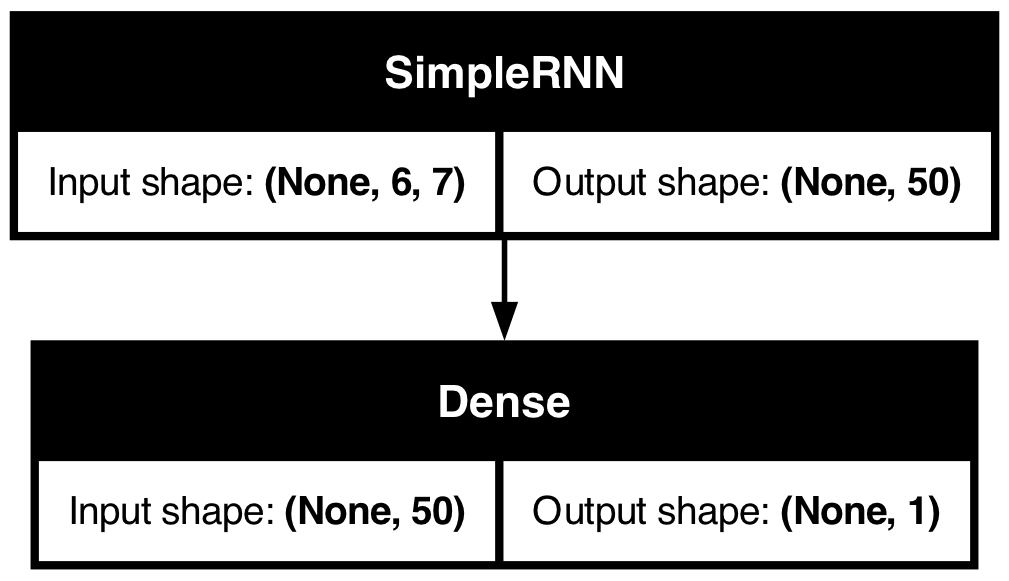
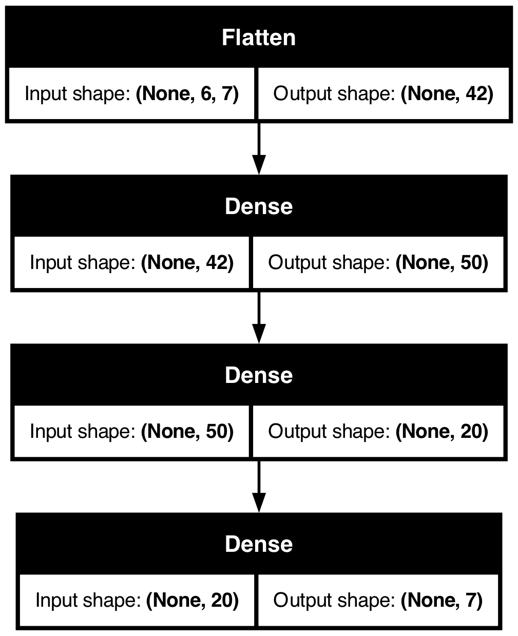
Plot the model

from keras.utils import plot_model

plot_model(model_dense, show_shapes=True)

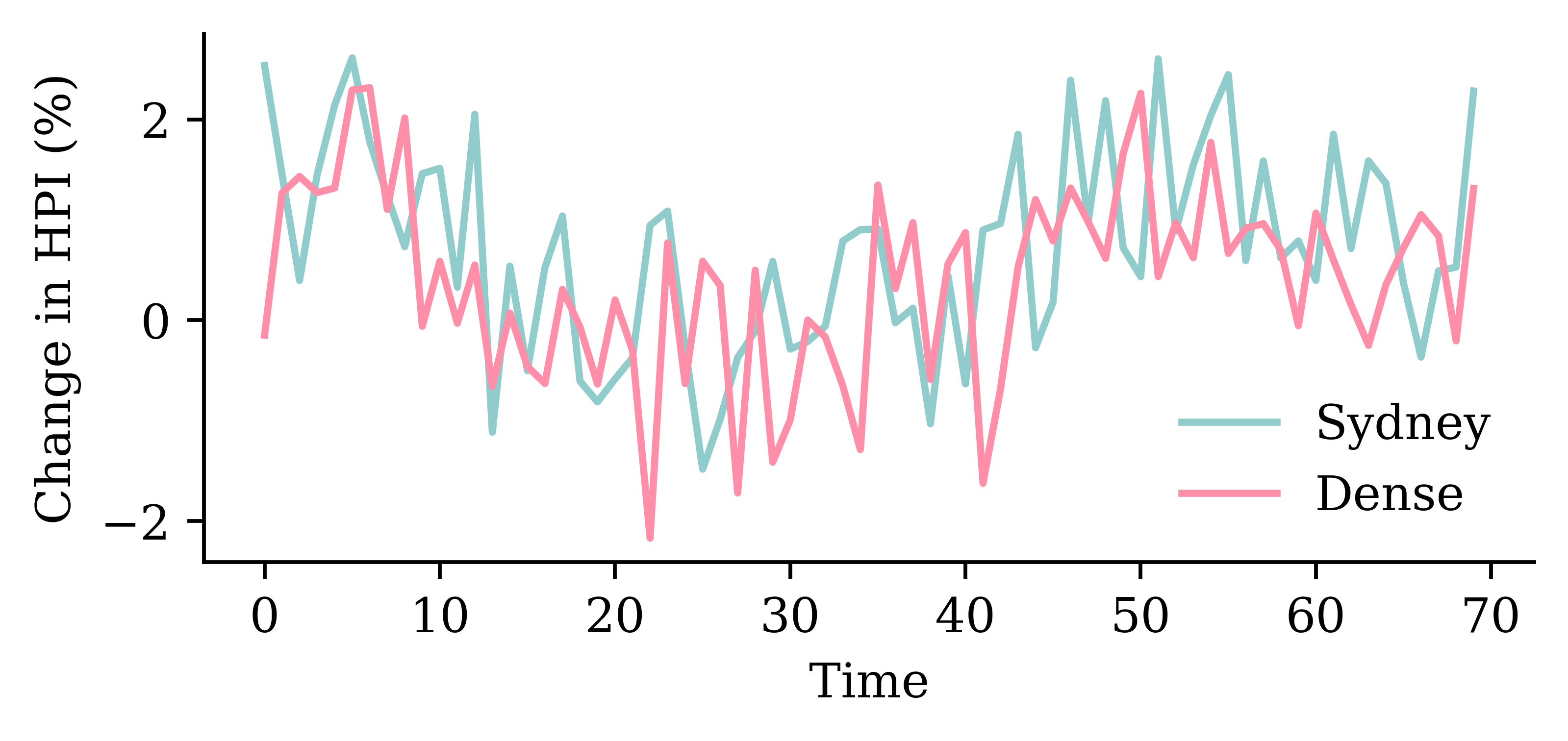
Assess the fits

model_dense.evaluate(X_val, y_val, verbose=0)

1.3529319763183594

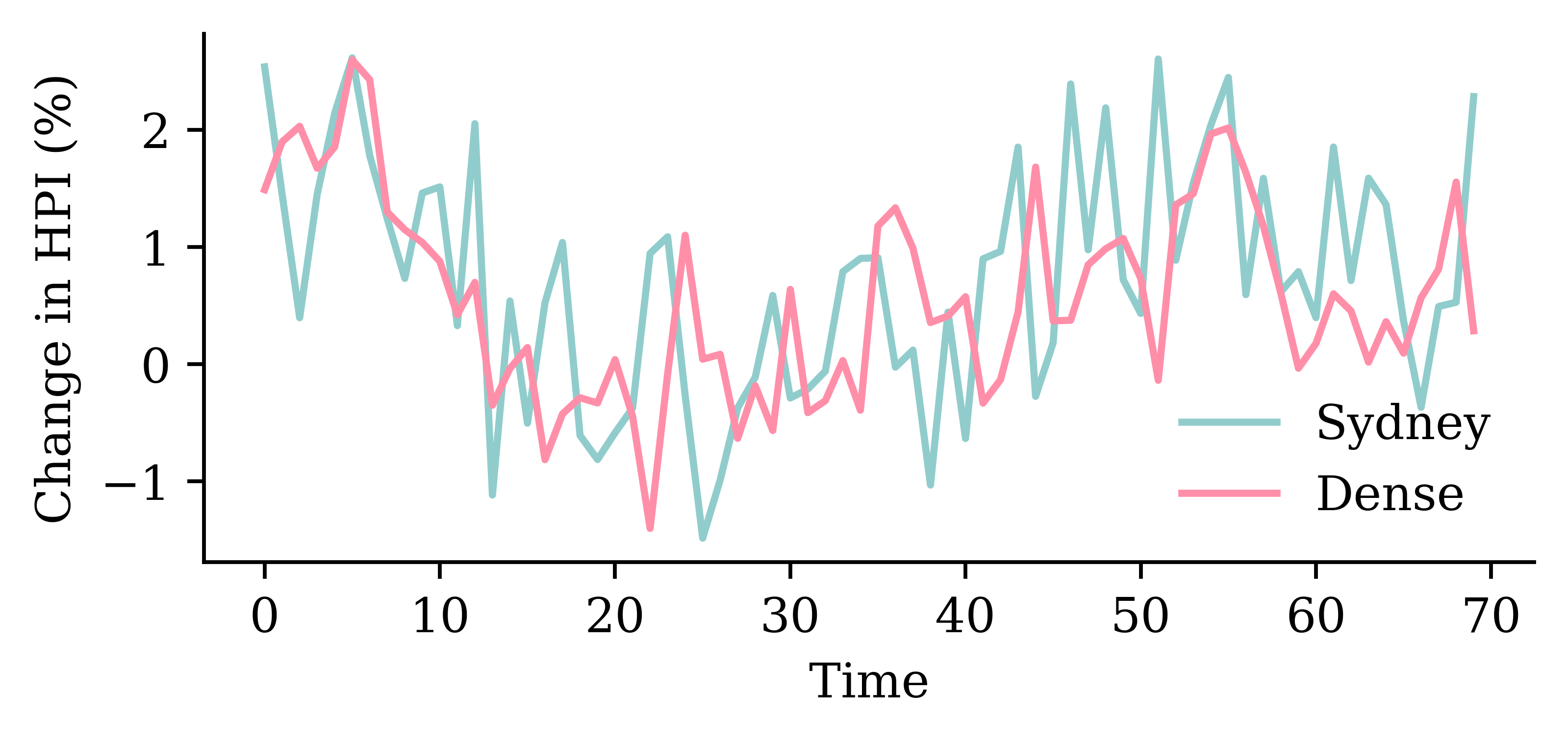
Code

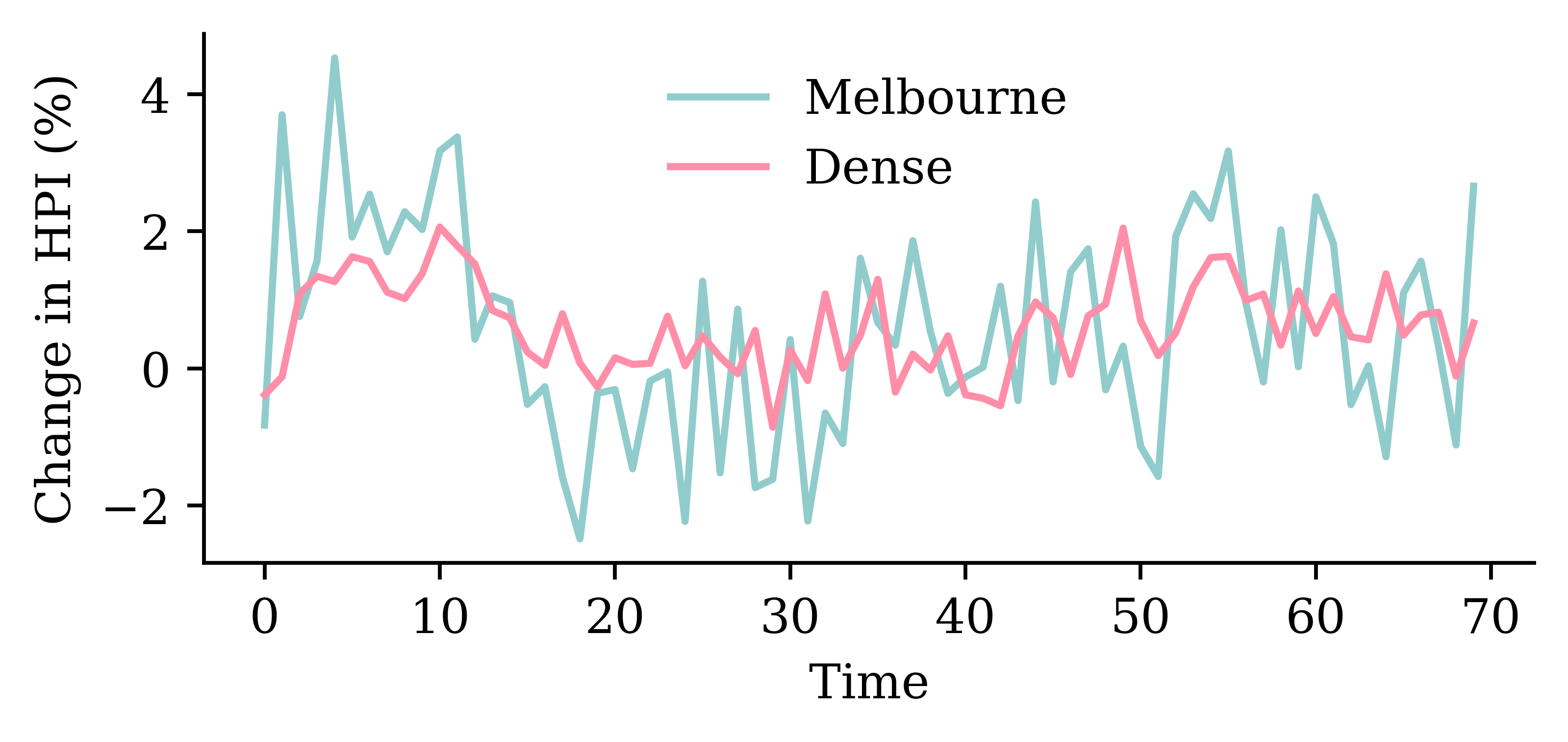
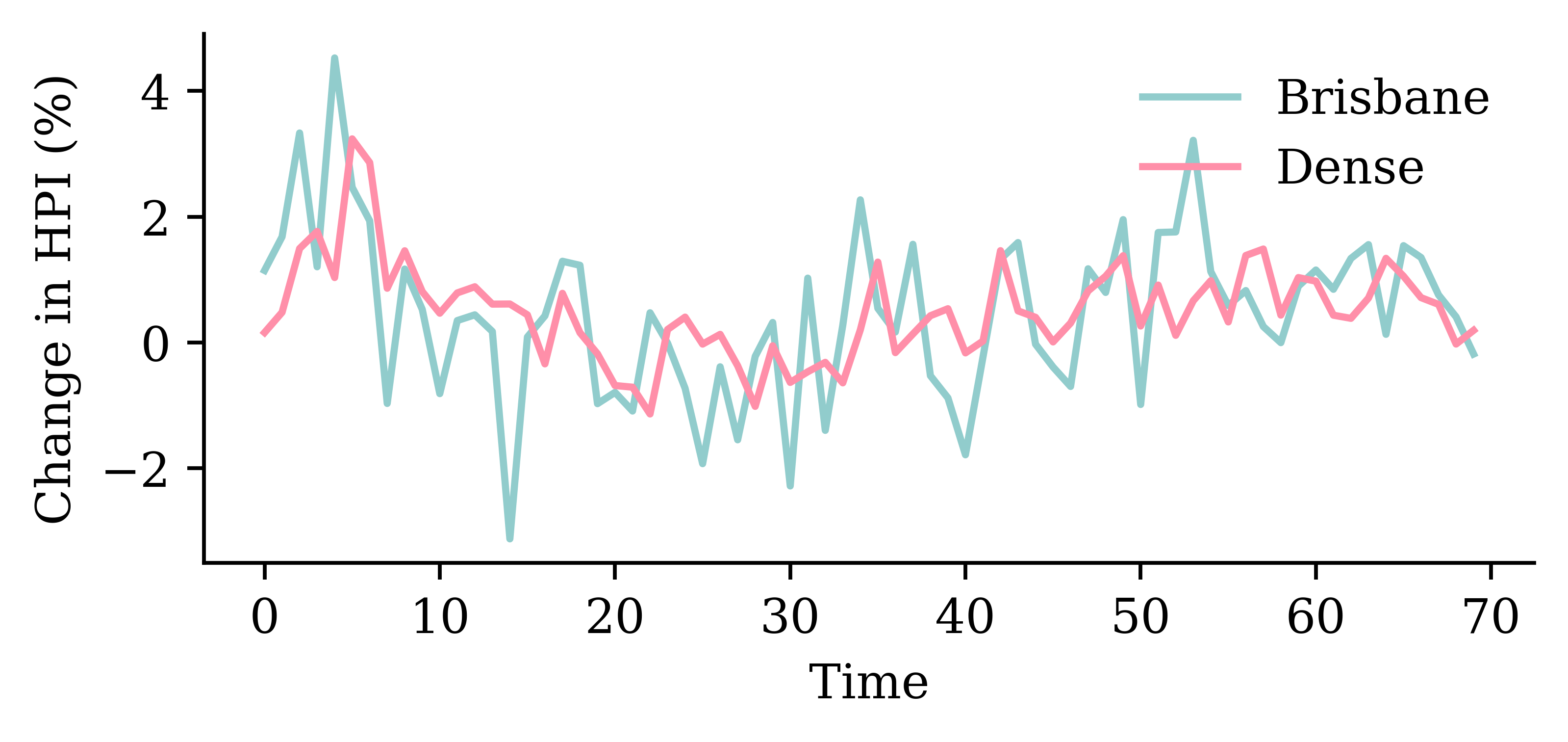
y_pred = model_dense.predict(X_val, verbose=0)
plt.plot(y_val, label="Sydney")
plt.plot(y_pred, label="Dense")
plt.xlabel("Time")
plt.ylabel("Change in HPI (%)")
plt.legend(frameon=False);

A `SimpleRNN` layer

random.seed(1)

model_simple = Sequential([
    Input((seq_length, num_ts)),
    SimpleRNN(50),
    Dense(1, activation="linear")
])
model_simple.compile(loss="mse", optimizer="adam")
print(f"This model has {model_simple.count_params()} parameters.")

es = EarlyStopping(patience=50, restore_best_weights=True, verbose=1)
%time hist = model_simple.fit(X_train, y_train, epochs=1_000, \
  validation_data=(X_val, y_val), callbacks=[es], verbose=0);

This model has 2951 parameters.
Epoch 53: early stopping
Restoring model weights from the end of the best epoch: 3.
CPU times: user 1.04 s, sys: 48.1 ms, total: 1.09 s
Wall time: 1.06 s

Plot the model

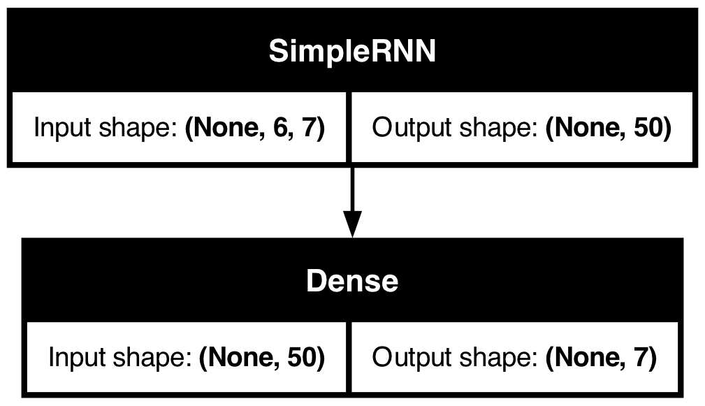
plot_model(model_simple, show_shapes=True)

Assess the fits

model_simple.evaluate(X_val, y_val, verbose=0)

0.8649981021881104

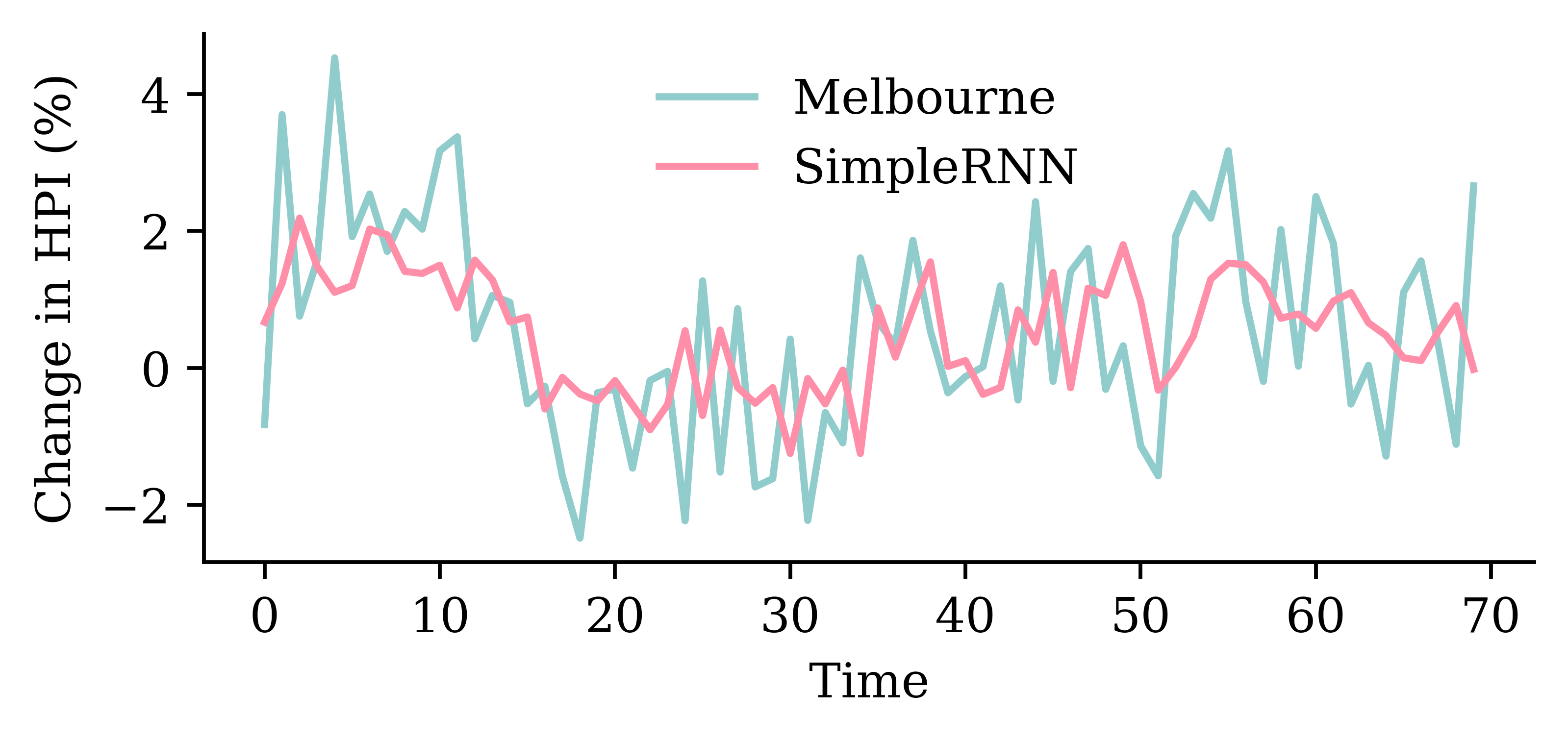
Code

y_pred = model_simple.predict(X_val, verbose=0)

plt.plot(y_val, label="Sydney")
plt.plot(y_pred, label="SimpleRNN")
plt.xlabel("Time")
plt.ylabel("Change in HPI (%)")
plt.legend(frameon=False);

A `LSTM` layer

from keras.layers import LSTM

random.seed(1)

model_lstm = Sequential([
    Input((seq_length, num_ts)),
    LSTM(50),
    Dense(1, activation="linear")
])

model_lstm.compile(loss="mse", optimizer="adam")

es = EarlyStopping(patience=50, restore_best_weights=True, verbose=1)

%time hist = model_lstm.fit(X_train, y_train, epochs=1_000, \
  validation_data=(X_val, y_val), callbacks=[es], verbose=0);

Epoch 58: early stopping
Restoring model weights from the end of the best epoch: 8.
CPU times: user 1.45 s, sys: 61.3 ms, total: 1.51 s
Wall time: 1.48 s

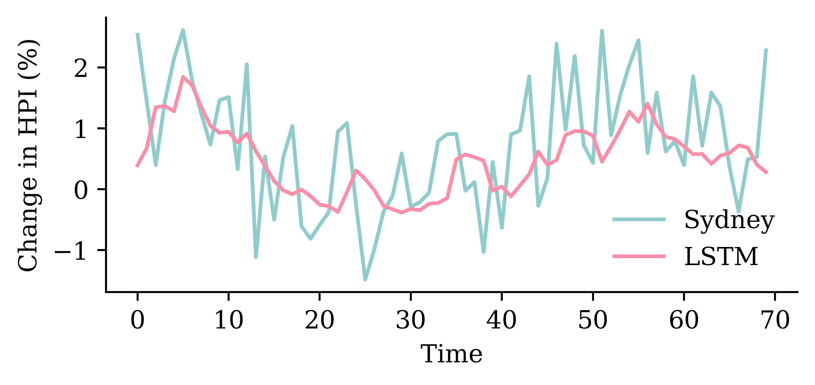
Assess the fits

model_lstm.evaluate(X_val, y_val, verbose=0)

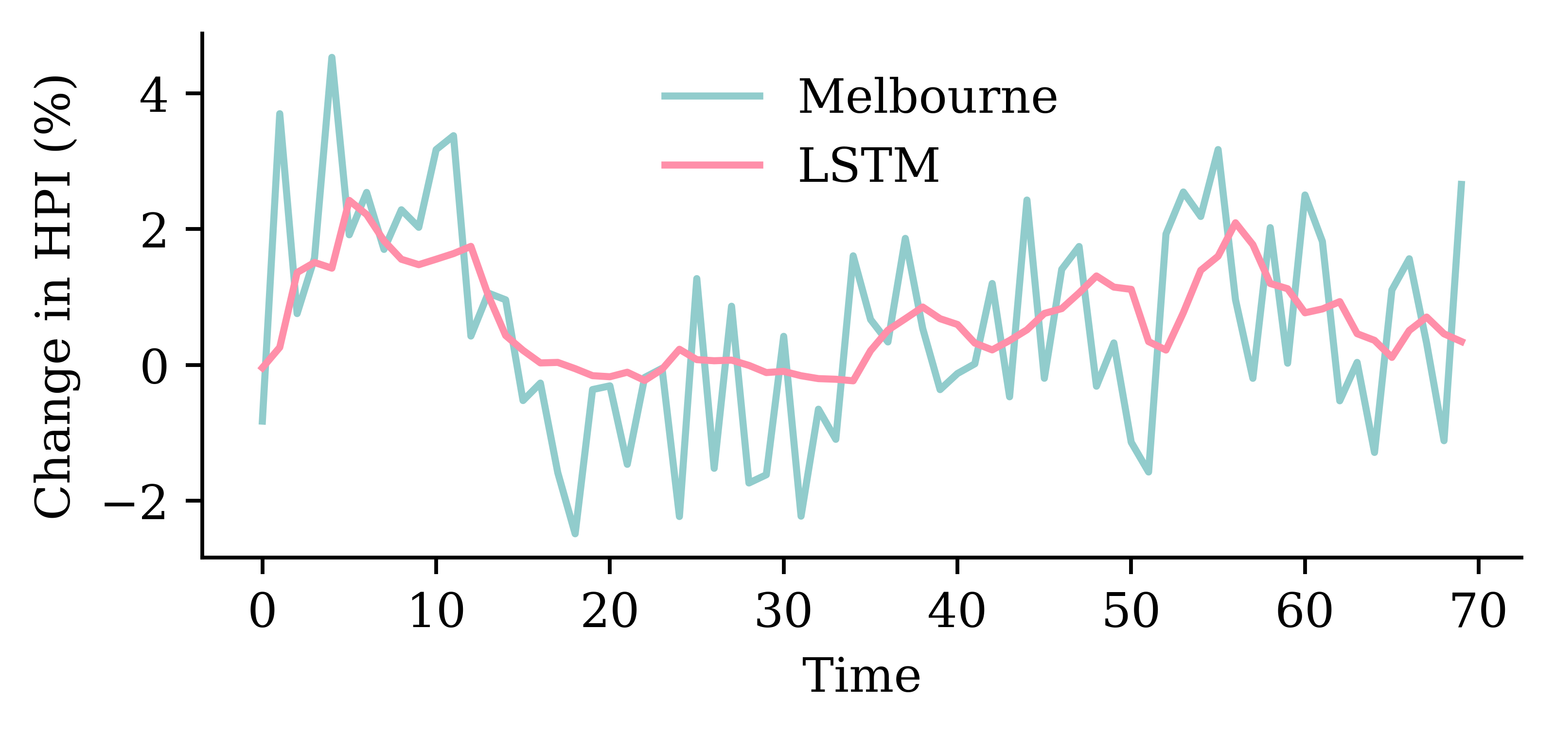
0.8229678273200989

Code

y_pred = model_lstm.predict(X_val, verbose=0)
plt.plot(y_val, label="Sydney")
plt.plot(y_pred, label="LSTM")
plt.xlabel("Time")
plt.ylabel("Change in HPI (%)")
plt.legend(frameon=False);

A `GRU` layer

from keras.layers import GRU

random.seed(1)

model_gru = Sequential([
    Input((seq_length, num_ts)),
    GRU(50),
    Dense(1, activation="linear")
])

model_gru.compile(loss="mse", optimizer="adam")

es = EarlyStopping(patience=50, restore_best_weights=True, verbose=1)

%time hist = model_gru.fit(X_train, y_train, epochs=1_000, \
  validation_data=(X_val, y_val), callbacks=[es], verbose=0)

Epoch 59: early stopping
Restoring model weights from the end of the best epoch: 9.
CPU times: user 1.55 s, sys: 58.7 ms, total: 1.61 s
Wall time: 1.57 s

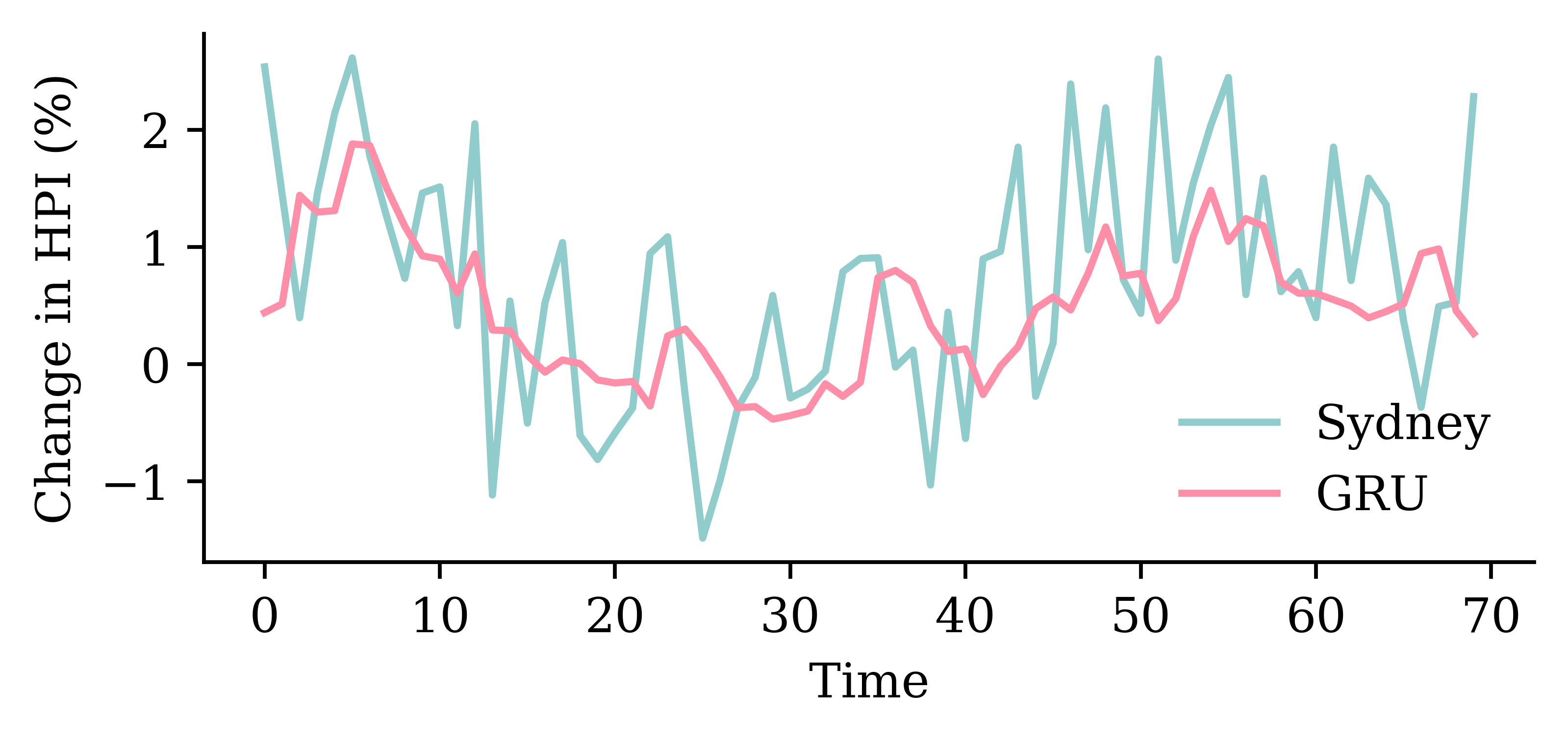
Assess the fits

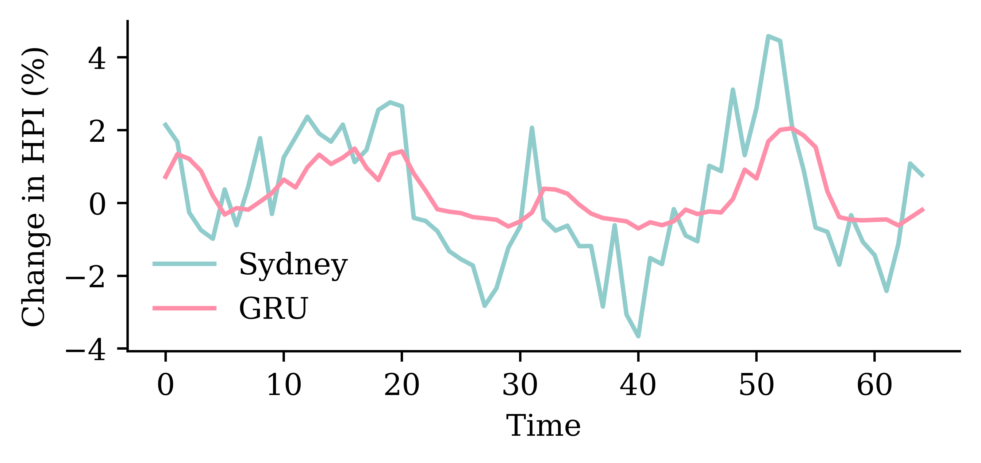
model_gru.evaluate(X_val, y_val, verbose=0)

0.813169002532959

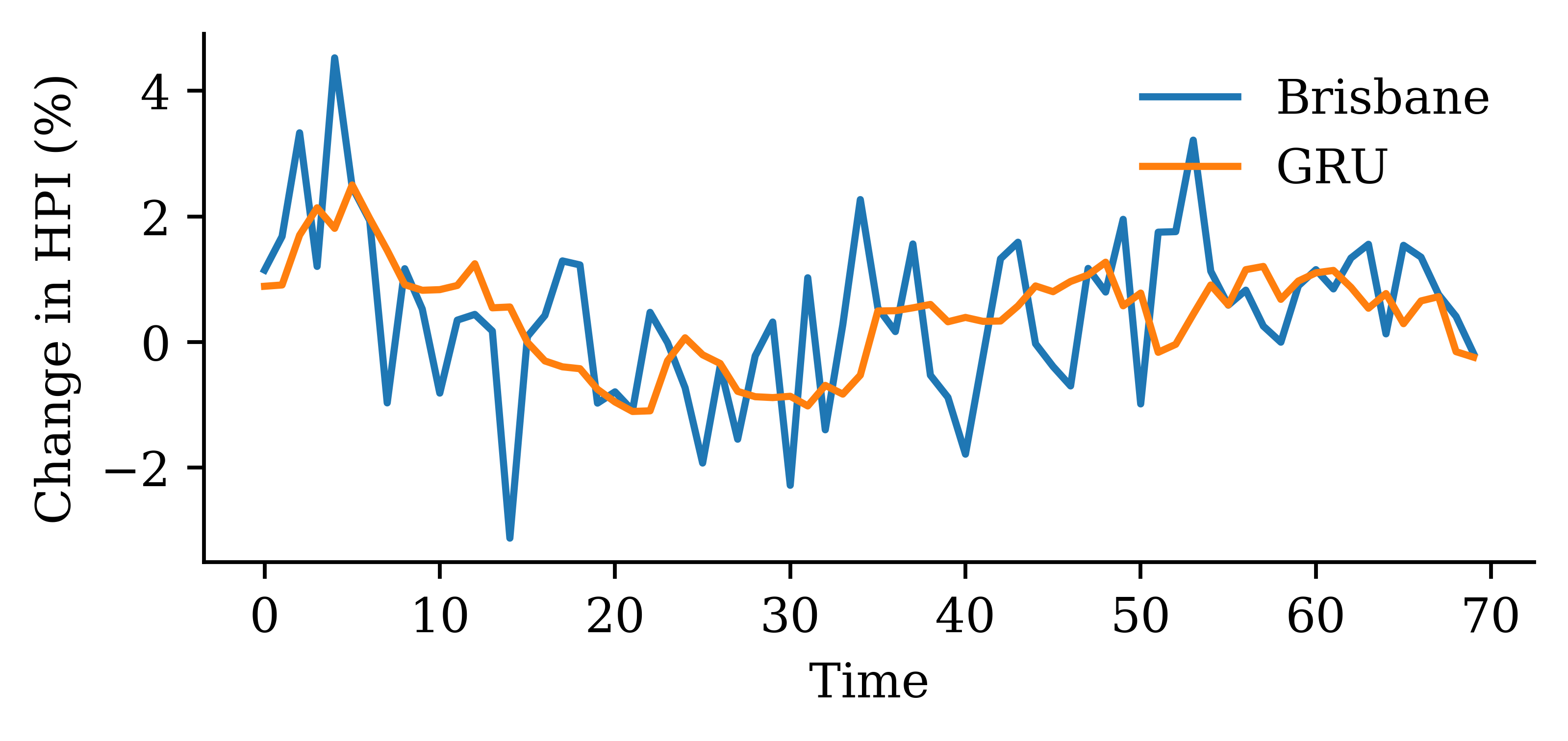
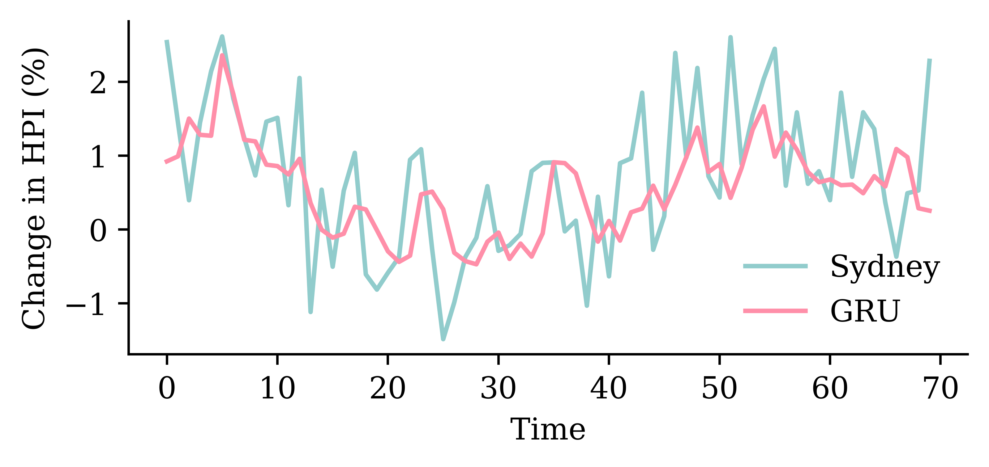
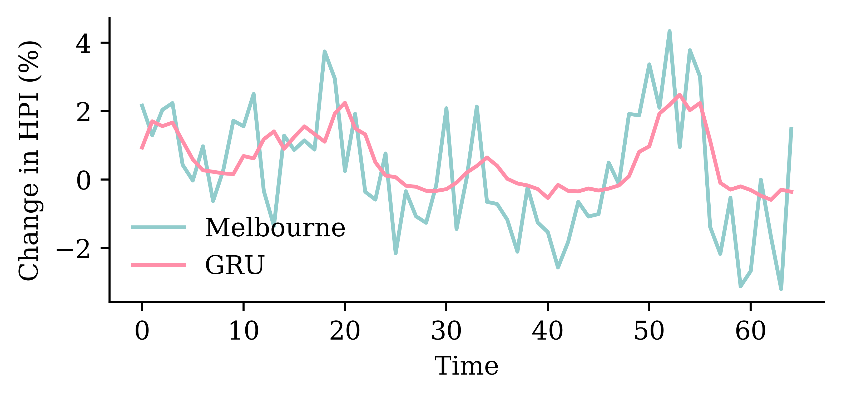
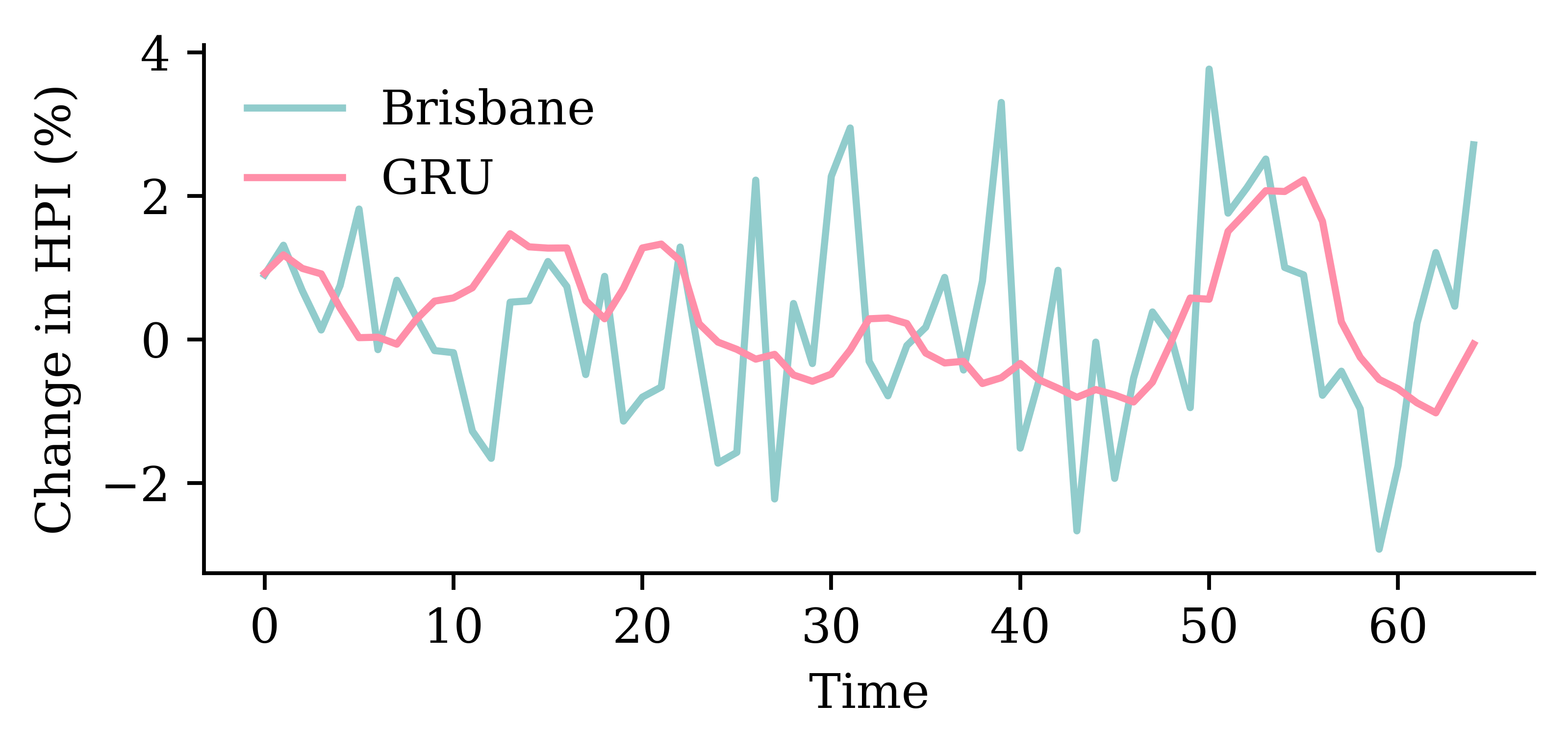
Code

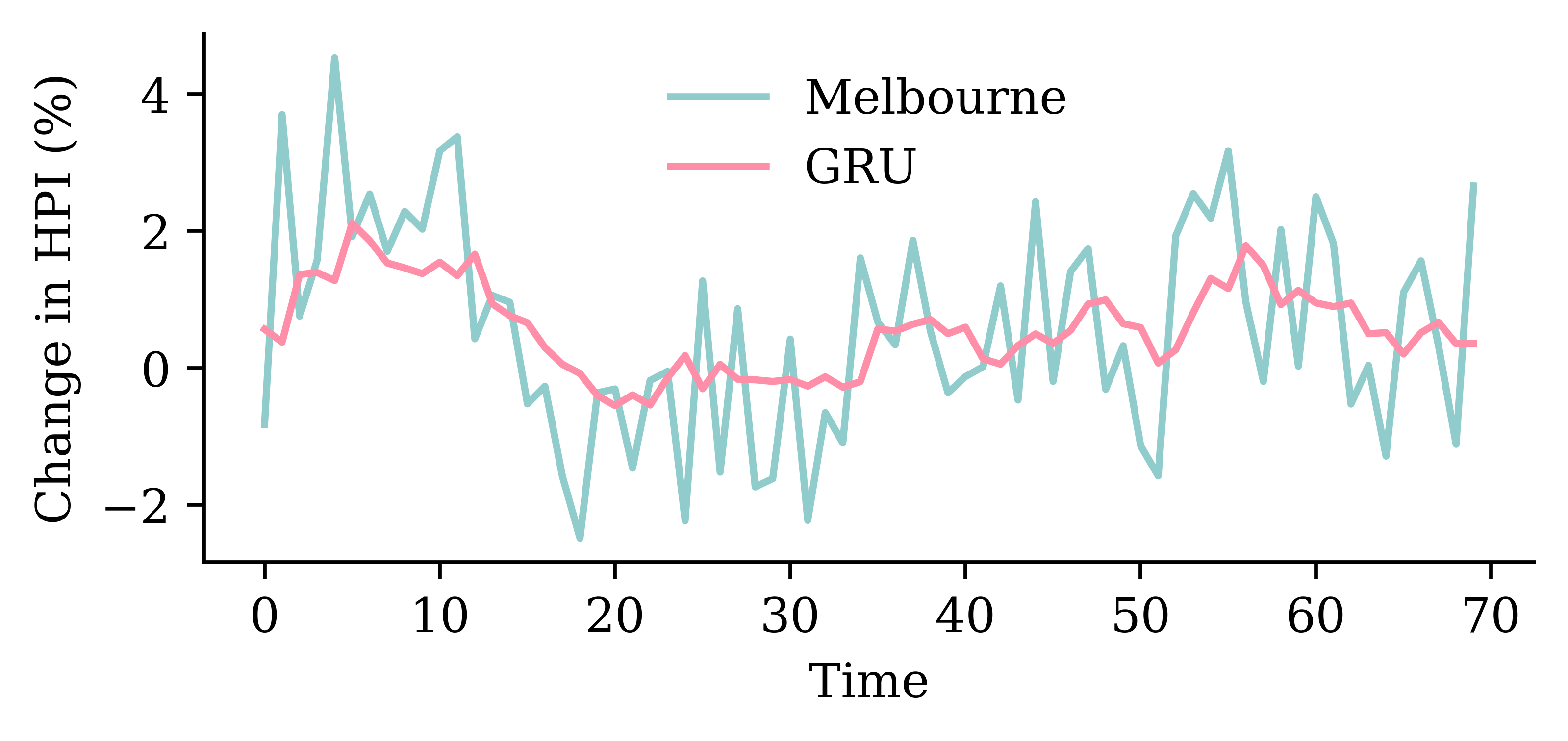
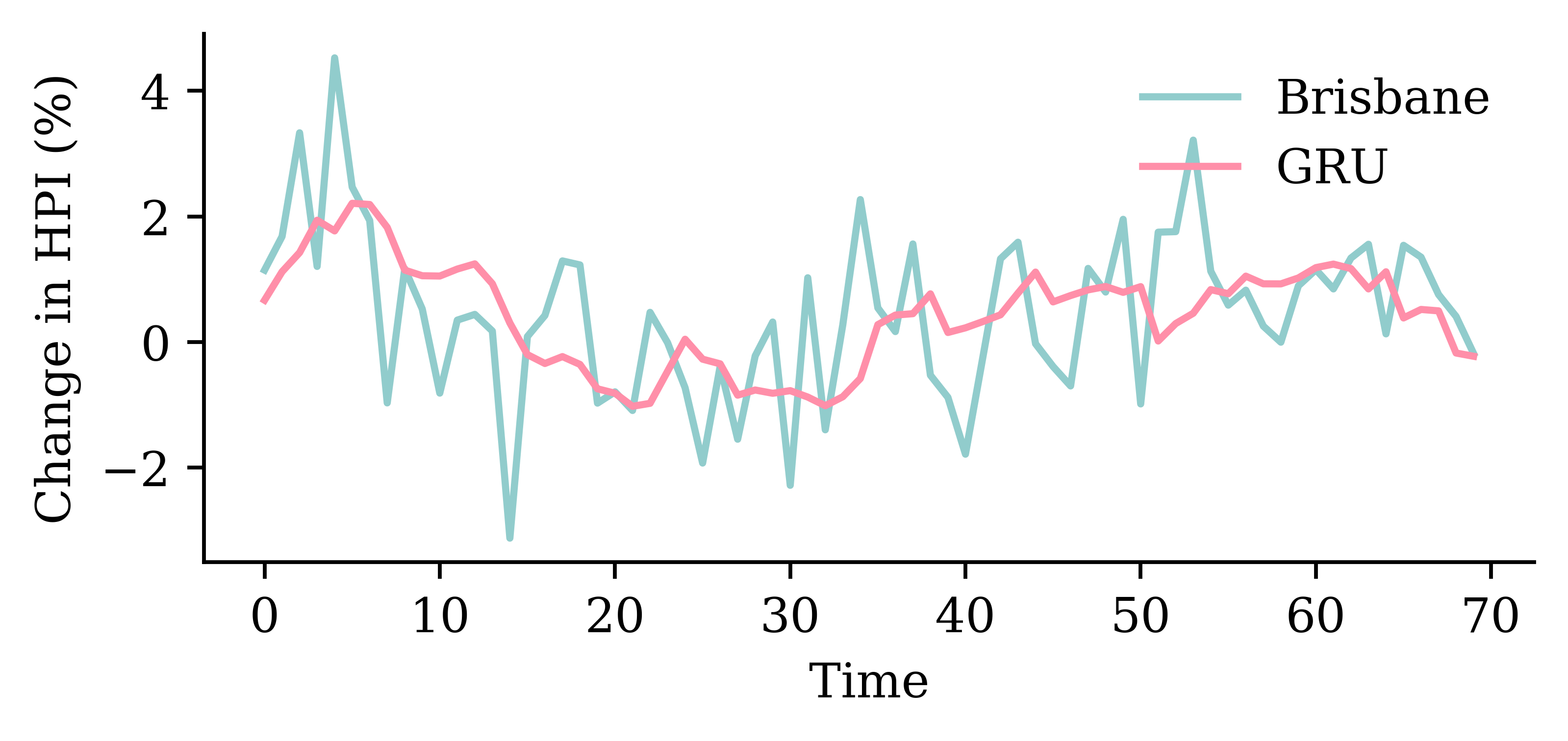
y_pred = model_gru.predict(X_val, verbose=0)
plt.plot(y_val, label="Sydney")
plt.plot(y_pred, label="GRU")
plt.xlabel("Time")
plt.ylabel("Change in HPI (%)")
plt.legend(frameon=False);

Two `GRU` layers

random.seed(1)

model_two_grus = Sequential([
    Input((seq_length, num_ts)),
    GRU(50, return_sequences=True),
    GRU(50),
    Dense(1, activation="linear")
])

model_two_grus.compile(loss="mse", optimizer="adam")

es = EarlyStopping(patience=50, restore_best_weights=True, verbose=1)

%time hist = model_two_grus.fit(X_train, y_train, epochs=1_000, \
  validation_data=(X_val, y_val), callbacks=[es], verbose=0)

Epoch 57: early stopping
Restoring model weights from the end of the best epoch: 7.
CPU times: user 2.56 s, sys: 105 ms, total: 2.66 s
Wall time: 2.6 s

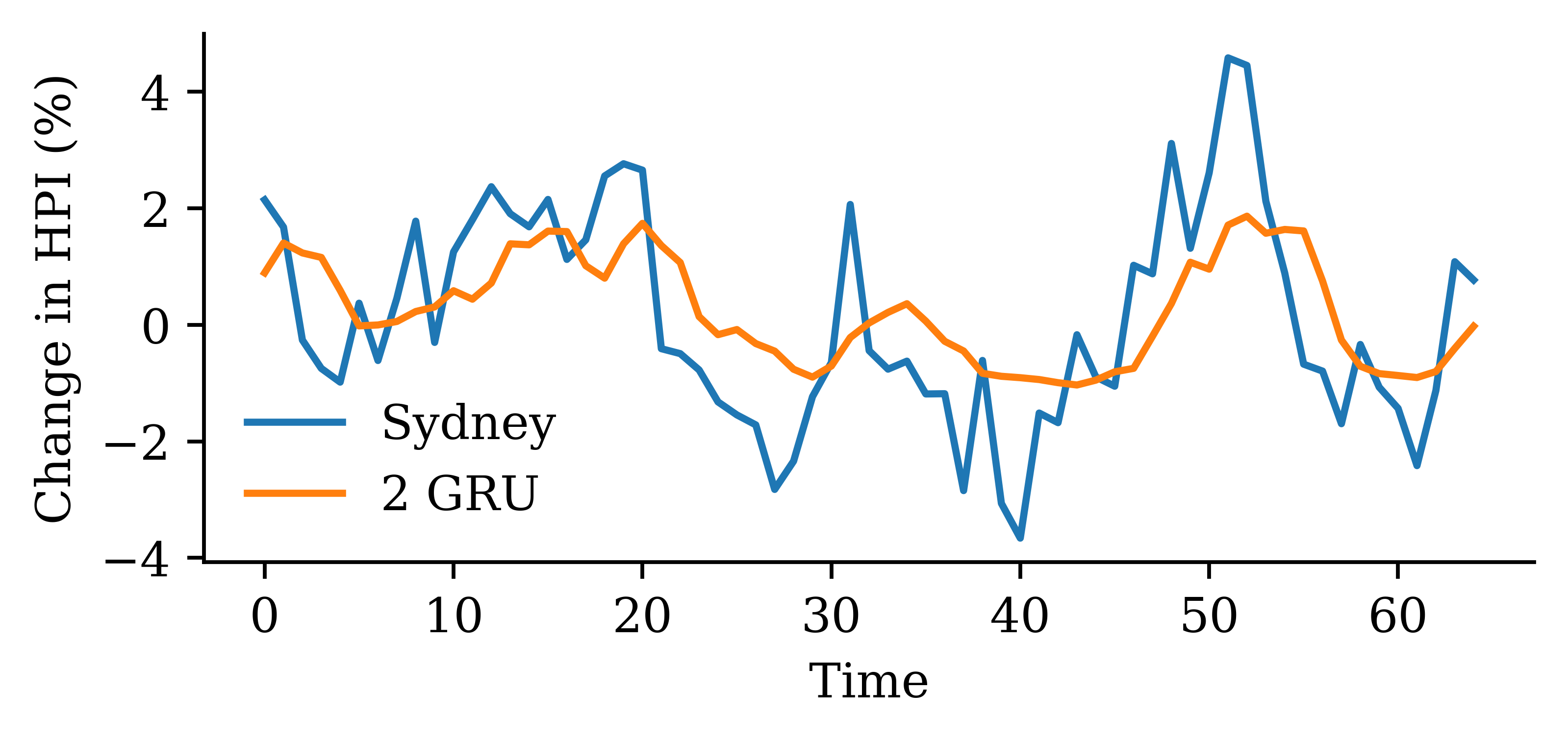
Assess the fits

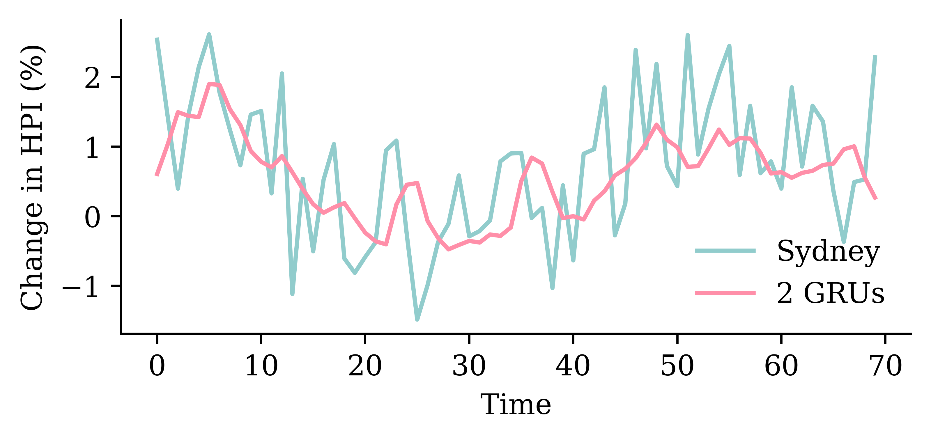
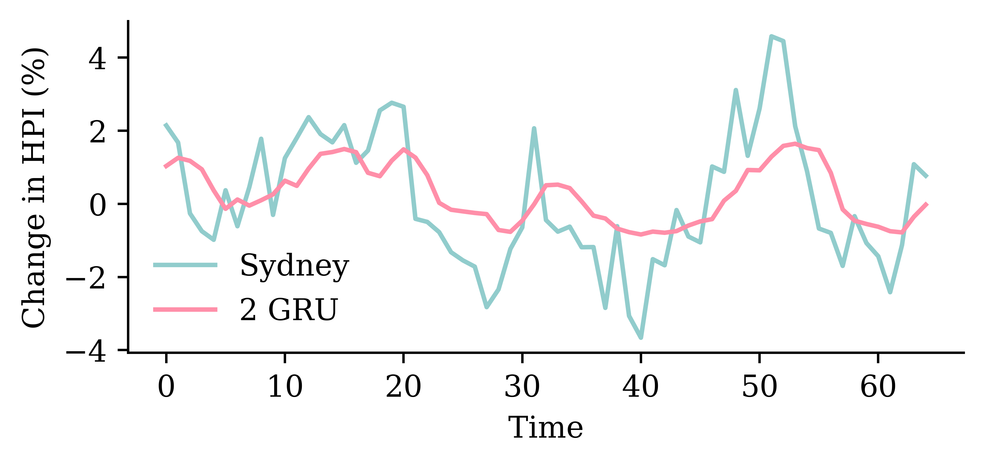
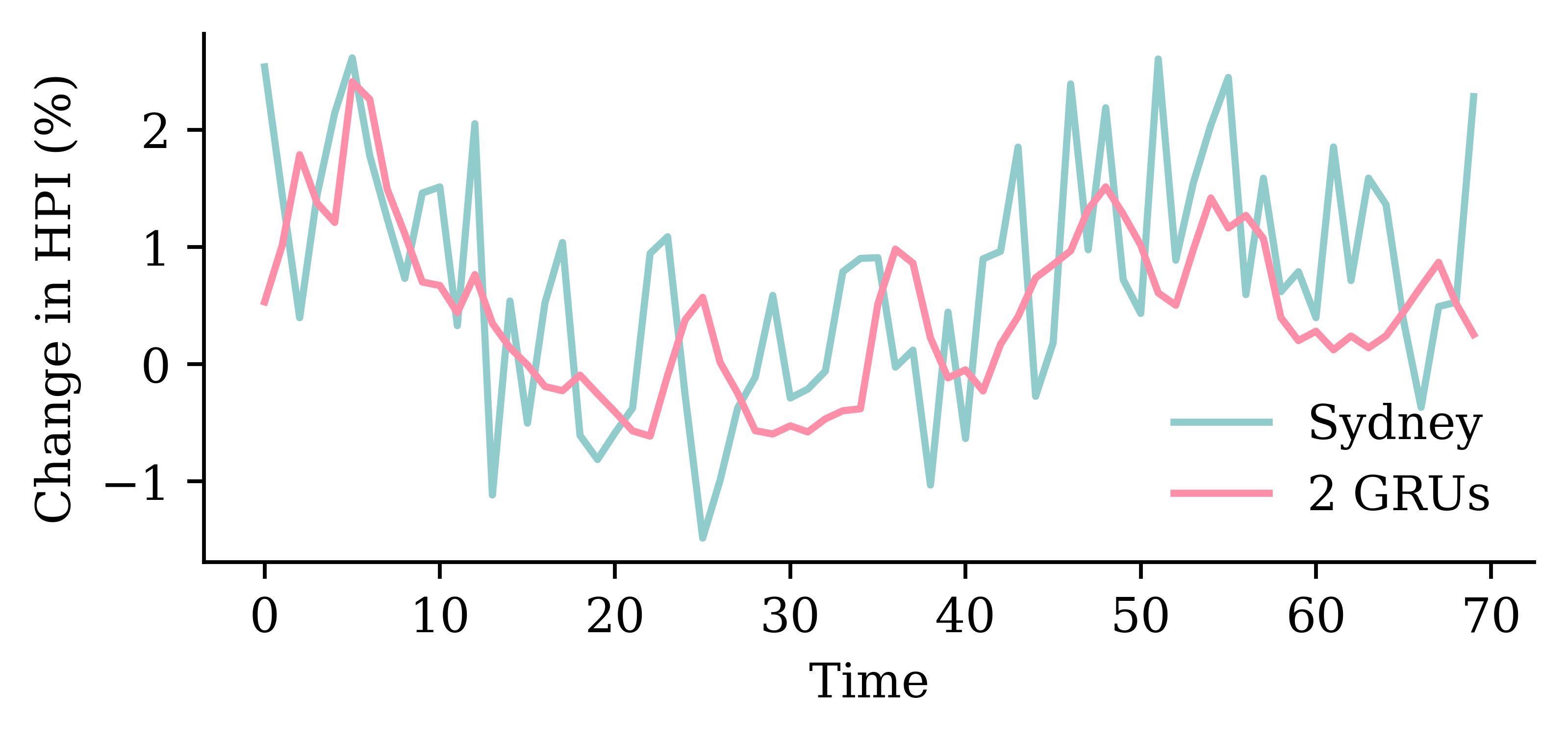
model_two_grus.evaluate(X_val, y_val, verbose=0)

0.7832801342010498

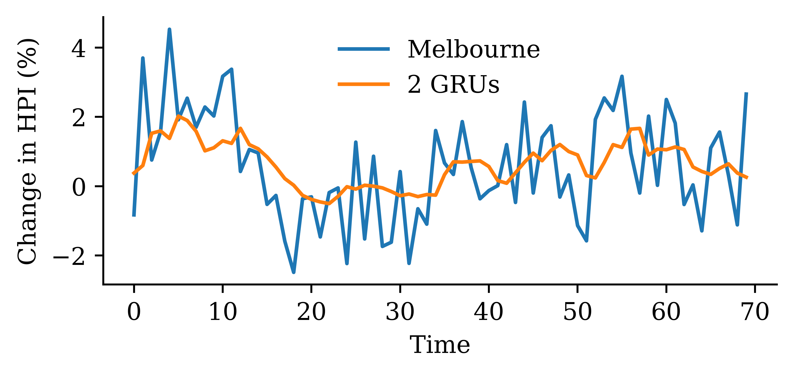
Code

y_pred = model_two_grus.predict(X_val, verbose=0)
plt.plot(y_val, label="Sydney")
plt.plot(y_pred, label="2 GRUs")
plt.xlabel("Time")
plt.ylabel("Change in HPI (%)")
plt.legend(frameon=False);

Compare the models

	Model	MSE
0	Dense	1.352932
1	SimpleRNN	0.864998
2	LSTM	0.822968
3	GRU	0.813169
4	2 GRUs	0.783280

The network with two GRU layers is the best.

model_two_grus.evaluate(X_test, y_test, verbose=0)

1.9257299900054932

Test set

Code

y_pred = model_two_grus.predict(X_test, verbose=0)
plt.plot(y_test, label="Sydney")
plt.plot(y_pred, label="2 GRU")
plt.xlabel("Time")
plt.ylabel("Change in HPI (%)")
plt.legend(frameon=False);

Predicting Multiple Time Series

Creating input arrays

Change the targets argument to include all the suburbs.

X_train, y_train = make_sequences(
    changes[:-delay], changes[delay:],
    seq_length, end_index=num_train,
)

X_val, y_val = make_sequences(
    changes[:-delay], changes[delay:],
    seq_length, start_index=num_train,
    end_index=num_train + num_val,
)

X_test, y_test = make_sequences(
    changes[:-delay], changes[delay:],
    seq_length, start_index=num_train + num_val,
)

Training set shape

The shape of our training set is now:

X_train.shape

(220, 6, 7)

y_train.shape

(220, 7)

A dense network

random.seed(1)
model_dense = Sequential([
    Input((seq_length, num_ts)),
    Flatten(),
    Dense(50, activation="leaky_relu"),
    Dense(20, activation="leaky_relu"),
    Dense(num_ts, activation="linear")
])
model_dense.compile(loss="mse", optimizer="adam")
print(f"This model has {model_dense.count_params()} parameters.")

es = EarlyStopping(patience=50, restore_best_weights=True, verbose=1)
%time hist = model_dense.fit(X_train, y_train, epochs=1_000, \
  validation_data=(X_val, y_val), callbacks=[es], verbose=0);

This model has 3317 parameters.
Epoch 70: early stopping
Restoring model weights from the end of the best epoch: 20.
CPU times: user 751 ms, sys: 51.8 ms, total: 803 ms
Wall time: 771 ms

Plot the model

plot_model(model_dense, show_shapes=True)

Assess the fits

model_dense.evaluate(X_val, y_val, verbose=0)

1.4135159254074097

Code

Y_pred = model_dense.predict(X_val, verbose=0)
plt.scatter(y_val, Y_pred)
add_diagonal_line()
plt.xlabel("Actual")
plt.ylabel("Predicted")
plt.show()

plt.plot(y_val[:, 4], label="Melbourne")
plt.plot(Y_pred[:, 4], label="Dense")
plt.xlabel("Time")
plt.ylabel("Change in HPI (%)")
plt.legend(frameon=False);

Code

plt.plot(y_val[:, 0], label="Brisbane")
plt.plot(Y_pred[:, 0], label="Dense")
plt.xlabel("Time")
plt.ylabel("Change in HPI (%)")
plt.legend(frameon=False)
plt.show()

plt.plot(y_val[:, 6], label="Sydney")
plt.plot(Y_pred[:, 6], label="Dense")
plt.xlabel("Time")
plt.ylabel("Change in HPI (%)")
plt.legend(frameon=False);

A `SimpleRNN` layer

random.seed(1)

model_simple = Sequential([
    Input((seq_length, num_ts)),
    SimpleRNN(50),
    Dense(num_ts, activation="linear")
])
model_simple.compile(loss="mse", optimizer="adam")
print(f"This model has {model_simple.count_params()} parameters.")

es = EarlyStopping(patience=50, restore_best_weights=True, verbose=1)
%time hist = model_simple.fit(X_train, y_train, epochs=1_000, \
  validation_data=(X_val, y_val), callbacks=[es], verbose=0);

This model has 3257 parameters.
Epoch 69: early stopping
Restoring model weights from the end of the best epoch: 19.
CPU times: user 1.3 s, sys: 57 ms, total: 1.36 s
Wall time: 1.32 s

Plot the model

plot_model(model_simple, show_shapes=True)

Assess the fits

model_simple.evaluate(X_val, y_val, verbose=0)

1.6102873086929321

Code

Y_pred = model_simple.predict(X_val, verbose=0)
plt.scatter(y_val, Y_pred)
add_diagonal_line()
plt.xlabel("Actual")
plt.ylabel("Predicted")
plt.show()

plt.plot(y_val[:, 4], label="Melbourne")
plt.plot(Y_pred[:, 4], label="SimpleRNN")
plt.xlabel("Time")
plt.ylabel("Change in HPI (%)")
plt.legend(frameon=False);

Code

plt.plot(y_val[:, 0], label="Brisbane")
plt.plot(Y_pred[:, 0], label="SimpleRNN")
plt.xlabel("Time")
plt.ylabel("Change in HPI (%)")
plt.legend(frameon=False)
plt.show()

plt.plot(y_val[:, 6], label="Sydney")
plt.plot(Y_pred[:, 6], label="SimpleRNN")
plt.xlabel("Time")
plt.ylabel("Change in HPI (%)")
plt.legend(frameon=False);

A `LSTM` layer

random.seed(1)

model_lstm = Sequential([
    Input((seq_length, num_ts)),
    LSTM(50),
    Dense(num_ts, activation="linear")
])

model_lstm.compile(loss="mse", optimizer="adam")

es = EarlyStopping(patience=50, restore_best_weights=True, verbose=1)

%time hist = model_lstm.fit(X_train, y_train, epochs=1_000, \
  validation_data=(X_val, y_val), callbacks=[es], verbose=0);

Epoch 76: early stopping
Restoring model weights from the end of the best epoch: 26.
CPU times: user 1.77 s, sys: 75.7 ms, total: 1.84 s
Wall time: 1.8 s

Assess the fits

model_lstm.evaluate(X_val, y_val, verbose=0)

1.3229057788848877

Code

Y_pred = model_lstm.predict(X_val, verbose=0)
plt.scatter(y_val, Y_pred)
add_diagonal_line()
plt.xlabel("Actual")
plt.ylabel("Predicted")
plt.show()

plt.plot(y_val[:, 4], label="Melbourne")
plt.plot(Y_pred[:, 4], label="LSTM")
plt.xlabel("Time")
plt.ylabel("Change in HPI (%)")
plt.legend(frameon=False);

Code

plt.plot(y_val[:, 0], label="Brisbane")
plt.plot(Y_pred[:, 0], label="LSTM")
plt.xlabel("Time")
plt.ylabel("Change in HPI (%)")
plt.legend(frameon=False)
plt.show()

plt.plot(y_val[:, 6], label="Sydney")
plt.plot(Y_pred[:, 6], label="LSTM")
plt.xlabel("Time")
plt.ylabel("Change in HPI (%)")
plt.legend(frameon=False);

A `GRU` layer

random.seed(1)

model_gru = Sequential([
    Input((seq_length, num_ts)),
    GRU(50),
    Dense(num_ts, activation="linear")
])

model_gru.compile(loss="mse", optimizer="adam")

es = EarlyStopping(patience=50, restore_best_weights=True, verbose=1)

%time hist = model_gru.fit(X_train, y_train, epochs=1_000, \
  validation_data=(X_val, y_val), callbacks=[es], verbose=0)

Epoch 69: early stopping
Restoring model weights from the end of the best epoch: 19.
CPU times: user 1.72 s, sys: 63.5 ms, total: 1.79 s
Wall time: 1.75 s

Assess the fits

model_gru.evaluate(X_val, y_val, verbose=0)

1.340381383895874

Code

Y_pred = model_gru.predict(X_val, verbose=0)
plt.scatter(y_val, Y_pred)
add_diagonal_line()
plt.xlabel("Actual")
plt.ylabel("Predicted")
plt.show()

plt.plot(y_val[:, 4], label="Melbourne")
plt.plot(Y_pred[:, 4], label="GRU")
plt.xlabel("Time")
plt.ylabel("Change in HPI (%)")
plt.legend(frameon=False);

Code

plt.plot(y_val[:, 0], label="Brisbane")
plt.plot(Y_pred[:, 0], label="GRU")
plt.xlabel("Time")
plt.ylabel("Change in HPI (%)")
plt.legend(frameon=False)
plt.show()

plt.plot(y_val[:, 6], label="Sydney")
plt.plot(Y_pred[:, 6], label="GRU")
plt.xlabel("Time")
plt.ylabel("Change in HPI (%)")
plt.legend(frameon=False);

Two `GRU` layers

random.seed(1)

model_two_grus = Sequential([
    Input((seq_length, num_ts)),
    GRU(50, return_sequences=True),
    GRU(50),
    Dense(num_ts, activation="linear")
])

model_two_grus.compile(loss="mse", optimizer="adam")

es = EarlyStopping(patience=50, restore_best_weights=True, verbose=1)

%time hist = model_two_grus.fit(X_train, y_train, epochs=1_000, \
  validation_data=(X_val, y_val), callbacks=[es], verbose=0)

Epoch 74: early stopping
Restoring model weights from the end of the best epoch: 24.
CPU times: user 3.15 s, sys: 123 ms, total: 3.27 s
Wall time: 3.2 s

Assess the fits

model_two_grus.evaluate(X_val, y_val, verbose=0)

1.3471126556396484

Code

Y_pred = model_two_grus.predict(X_val, verbose=0)
plt.scatter(y_val, Y_pred)
add_diagonal_line()
plt.xlabel("Actual")
plt.ylabel("Predicted")
plt.show()

plt.plot(y_val[:, 4], label="Melbourne")
plt.plot(Y_pred[:, 4], label="2 GRUs")
plt.xlabel("Time")
plt.ylabel("Change in HPI (%)")
plt.legend(frameon=False);

Code

plt.plot(y_val[:, 0], label="Brisbane")
plt.plot(Y_pred[:, 0], label="2 GRUs")
plt.xlabel("Time")
plt.ylabel("Change in HPI (%)")
plt.legend(frameon=False)
plt.show()

plt.plot(y_val[:, 6], label="Sydney")
plt.plot(Y_pred[:, 6], label="2 GRUs")
plt.xlabel("Time")
plt.ylabel("Change in HPI (%)")
plt.legend(frameon=False);

Compare the models

Code

models = [model_dense, model_simple, model_lstm, model_gru, model_two_grus]
model_names = ["Dense", "SimpleRNN", "LSTM", "GRU", "2 GRUs"]
mse_val = {
    name: model.evaluate(X_val, y_val, verbose=0)
    for name, model in zip(model_names, models)
}
val_results = pd.DataFrame({"Model": mse_val.keys(), "MSE": mse_val.values()})
val_results.sort_values("MSE", ascending=False)

	Model	MSE
1	SimpleRNN	1.610287
0	Dense	1.413516
4	2 GRUs	1.347113
3	GRU	1.340381
2	LSTM	1.322906

The network with an LSTM layer is the best.

model_lstm.evaluate(X_test, y_test, verbose=0)

1.8732062578201294

Test set

Code

Y_pred = model_lstm.predict(X_test, verbose=0)
plt.scatter(y_test, Y_pred)
add_diagonal_line()
plt.xlabel("Actual")
plt.ylabel("Predicted")
plt.show()

plt.plot(y_test[:, 4], label="Melbourne")
plt.plot(Y_pred[:, 4], label="GRU")
plt.xlabel("Time")
plt.ylabel("Change in HPI (%)")
plt.legend(frameon=False);

Code

plt.plot(y_test[:, 0], label="Brisbane")
plt.plot(Y_pred[:, 0], label="GRU")
plt.xlabel("Time")
plt.ylabel("Change in HPI (%)")
plt.legend(frameon=False)
plt.show()

plt.plot(y_test[:, 6], label="Sydney")
plt.plot(Y_pred[:, 6], label="GRU")
plt.xlabel("Time")
plt.ylabel("Change in HPI (%)")
plt.legend(frameon=False);

Package Versions

from watermark import watermark
print(watermark(python=True, packages="keras,matplotlib,numpy,pandas,seaborn,scipy,torch"))

Python implementation: CPython
Python version       : 3.13.11
IPython version      : 9.10.0

keras     : 3.10.0
matplotlib: 3.10.0
numpy     : 2.4.2
pandas    : 3.0.0
seaborn   : 0.13.2
scipy     : 1.17.0
torch     : 2.10.0

Glossary

autoregressive forecasting
forecasting
GRU
LSTM
one-step/multi-step ahead forecasting
persistence forecast
recurrent neural networks
SimpleRNN