Classification

ACTL3143 & ACTL5111 Deep Learning for Actuaries

import random
from pathlib import Path

import matplotlib.pyplot as plt
import numpy as np
import pandas as pd
import seaborn as sns

from keras.models import Sequential
from keras.layers import Dense, Input
from keras.callbacks import EarlyStopping

from sklearn.model_selection import train_test_split
from sklearn.preprocessing import OneHotEncoder, StandardScaler
from sklearn.compose import make_column_transformer
from sklearn.impute import SimpleImputer
from sklearn import set_config

set_config(transform_output="pandas")

Example 1: Binary Classification

Stroke Prediction Data description

1. id: unique identifier
2. gender: “Male”, “Female” or “Other”
3. age: age of the patient
4. hypertension: 0 or 1 if the patient has hypertension
5. heart_disease: 0 or 1 if the patient has any heart disease
6. ever_married: “No” or “Yes”
7. work_type: “children”, “Govt_jov”, “Never_worked”, “Private” or “Self-employed”

8. Residence_type: “Rural” or “Urban”
9. avg_glucose_level: average glucose level in blood
10. bmi: body mass index
11. smoking_status: “formerly smoked”, “never smoked”, “smokes” or “Unknown”
12. stroke: 0 or 1 if the patient had a stroke

Source: Kaggle, Stroke Prediction Dataset.

Load up the (pre-)preprocessed data

PROCESSED_DATA_DIR = Path("stroke/processed")

X_train = pd.read_csv(PROCESSED_DATA_DIR / "x_train.csv")
X_val= pd.read_csv(PROCESSED_DATA_DIR / "x_val.csv")
X_test = pd.read_csv(PROCESSED_DATA_DIR / "x_test.csv")
y_train = pd.read_csv(PROCESSED_DATA_DIR / "y_train.csv")
y_val = pd.read_csv(PROCESSED_DATA_DIR / "y_val.csv")
y_test = pd.read_csv(PROCESSED_DATA_DIR / "y_test.csv")

X_train

	gender_Female	gender_Male	ever_married_No	ever_married_Yes	Residence_type_Rural	Residence_type_Urban	work_type_Govt_job	work_type_Never_worked	work_type_Private	work_type_Self-employed	work_type_children	smoking_status_Unknown	smoking_status_formerly smoked	smoking_status_never smoked	smoking_status_smokes	hypertension	heart_disease	age	avg_glucose_level	bmi
0	0.0	1.0	0.0	1.0	1.0	0.0	0.0	0.0	1.0	0.0	0.0	0.0	0.0	1.0	0.0	0	0	0.003896	-0.628661	0.005109
1	0.0	1.0	1.0	0.0	1.0	0.0	0.0	0.0	0.0	0.0	1.0	1.0	0.0	0.0	0.0	0	0	-1.634096	-0.257346	-1.509505
2	0.0	1.0	1.0	0.0	1.0	0.0	0.0	0.0	1.0	0.0	0.0	0.0	0.0	1.0	0.0	0	0	-0.483075	-0.754323	-0.732780
...	...	...	...	...	...	...	...	...	...	...	...	...	...	...	...	...	...	...	...	...
3063	1.0	0.0	0.0	1.0	1.0	0.0	1.0	0.0	0.0	0.0	0.0	0.0	0.0	1.0	0.0	1	0	0.667946	-1.028773	0.561761
3064	1.0	0.0	0.0	1.0	1.0	0.0	0.0	0.0	1.0	0.0	0.0	0.0	1.0	0.0	0.0	0	0	-0.084644	-0.366428	0.548816
3065	0.0	1.0	1.0	0.0	0.0	1.0	0.0	0.0	1.0	0.0	0.0	1.0	0.0	0.0	0.0	0	0	-1.147126	-0.765668	-0.422090

3066 rows × 20 columns

Target variable

y_train

	stroke
0	0
1	0
2	0
...	...
3063	0
3064	0
3065	0

3066 rows × 1 columns

import numpy as np
classes, counts = np.unique(y_train.values.ravel(), return_counts=True)
print("Classes:", classes)
print("Counts:", counts)

Classes: [0 1]
Counts: [2909  157]

This shows the distribution of the binary stroke target (0 = no stroke, 1 = stroke).

Setup a binary classification model

def create_model(seed=42):
    random.seed(seed)
    model = Sequential()
    model.add(Input(X_train.shape[1:]))
    model.add(Dense(32, "leaky_relu"))
    model.add(Dense(16, "leaky_relu"))
    model.add(Dense(1, "sigmoid"))
    return model

Since this is a binary classification problem, we use the sigmoid activation function.

model = create_model()
model.summary()

Model: "sequential"

┏━━━━━━━━━━━━━━━━━━━━━━━━━━━━━━━━━┳━━━━━━━━━━━━━━━━━━━━━━━━┳━━━━━━━━━━━━━━━┓
┃ Layer (type)                    ┃ Output Shape           ┃       Param # ┃
┡━━━━━━━━━━━━━━━━━━━━━━━━━━━━━━━━━╇━━━━━━━━━━━━━━━━━━━━━━━━╇━━━━━━━━━━━━━━━┩
│ dense (Dense)                   │ (None, 32)             │           672 │
├─────────────────────────────────┼────────────────────────┼───────────────┤
│ dense_1 (Dense)                 │ (None, 16)             │           528 │
├─────────────────────────────────┼────────────────────────┼───────────────┤
│ dense_2 (Dense)                 │ (None, 1)              │            17 │
└─────────────────────────────────┴────────────────────────┴───────────────┘

 Total params: 1,217 (4.75 KB)

 Trainable params: 1,217 (4.75 KB)

 Non-trainable params: 0 (0.00 B)

model.summary() returns the summary of the constructed neural network.

Fit the model

model = create_model()
model.compile("adam", "binary_crossentropy")
model.fit(X_train, y_train, epochs=5, verbose=2)

Epoch 1/5
96/96 - 0s - 4ms/step - loss: 0.2732
Epoch 2/5
96/96 - 0s - 643us/step - loss: 0.1701
Epoch 3/5
96/96 - 0s - 636us/step - loss: 0.1632
Epoch 4/5
96/96 - 0s - 696us/step - loss: 0.1603
Epoch 5/5
96/96 - 0s - 659us/step - loss: 0.1587

<keras.src.callbacks.history.History at 0x167dd8050>

This trains the model for 5 epochs without tracking any metrics.

Track accuracy as the model trains

model = create_model()
model.compile("adam", "binary_crossentropy", metrics=["accuracy"])
model.fit(X_train, y_train, epochs=5, verbose=2)

Epoch 1/5
96/96 - 0s - 4ms/step - accuracy: 0.9393 - loss: 0.2732
Epoch 2/5
96/96 - 0s - 727us/step - accuracy: 0.9488 - loss: 0.1701
Epoch 3/5
96/96 - 0s - 676us/step - accuracy: 0.9488 - loss: 0.1632
Epoch 4/5
96/96 - 0s - 662us/step - accuracy: 0.9488 - loss: 0.1603
Epoch 5/5
96/96 - 0s - 667us/step - accuracy: 0.9488 - loss: 0.1587

<keras.src.callbacks.history.History at 0x16980f510>

Here we include accuracy as a metric to monitor during training.

Run a long fit

model = create_model()
model.compile("adam", "binary_crossentropy", metrics=["accuracy"])
%time hist = model.fit(X_train, y_train, epochs=500, validation_data=(X_val, y_val), verbose=False)

CPU times: user 53.2 s, sys: 5.55 s, total: 58.8 s
Wall time: 48.5 s

We fit for 500 epochs and track time.

Add early stopping

model = create_model()
model.compile("adam", "binary_crossentropy", metrics=["accuracy"])
es = EarlyStopping(restore_best_weights=True, patience=50, monitor="val_accuracy")
%time hist_es = model.fit(X_train, y_train, epochs=500, validation_data=(X_val, y_val), callbacks=[es], verbose=False)
print(f"Stopped after {len(hist_es.history['loss'])} epochs.")

CPU times: user 5.73 s, sys: 622 ms, total: 6.35 s
Wall time: 5.23 s
Stopped after 51 epochs.

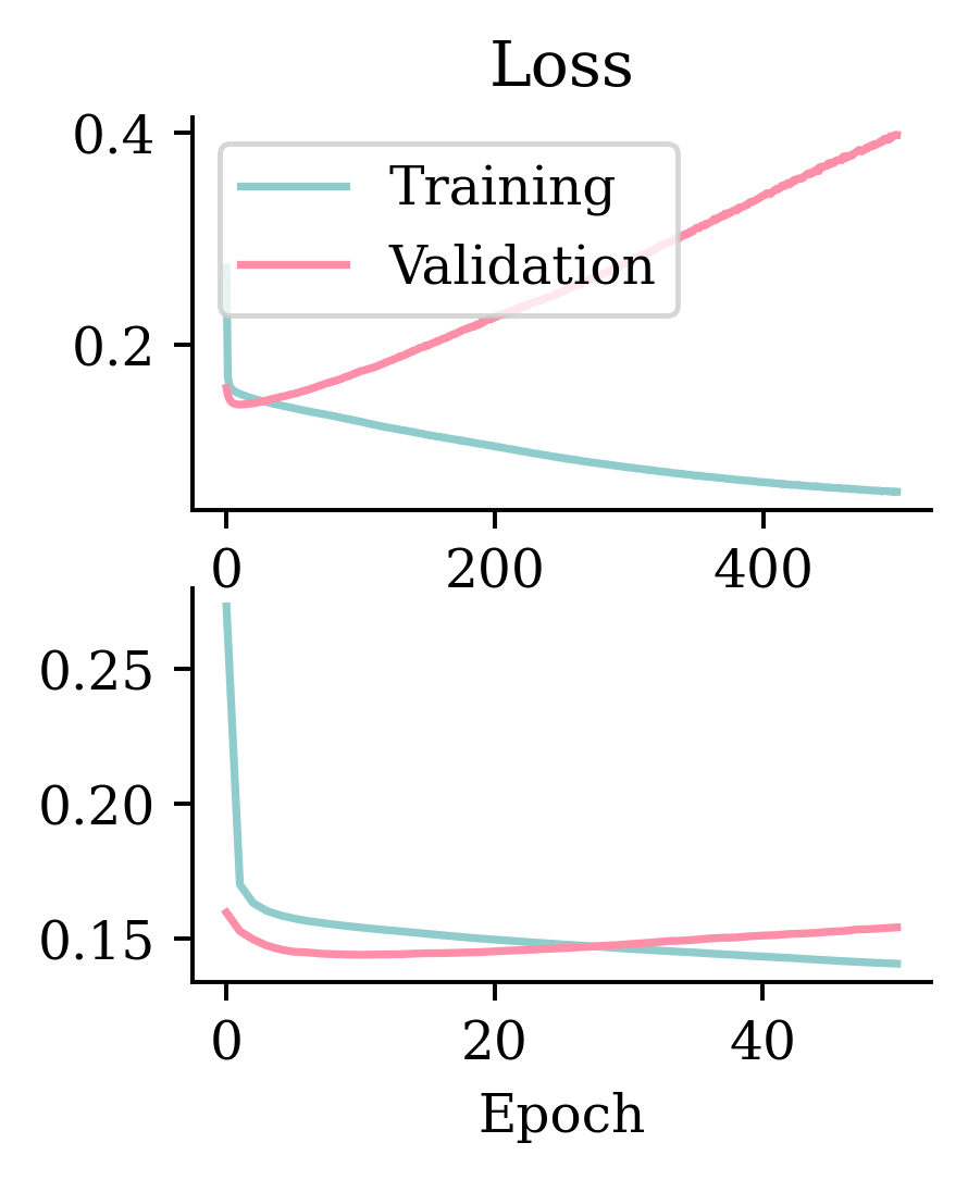
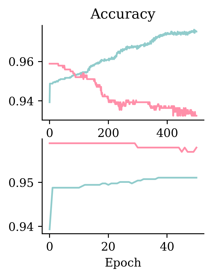
Early stopping is used to prevent overfitting by monitoring validation accuracy.

Fitting metrics

matplotlib.pyplot.rcParams["figure.figsize"] = (2.5, 2.95)
plt.subplot(2, 1, 1)
plt.plot(hist.history["loss"])
plt.plot(hist.history["val_loss"])
plt.title("Loss")
plt.legend(["Training", "Validation"])

plt.subplot(2, 1, 2)
plt.plot(hist_es.history["loss"])
plt.plot(hist_es.history["val_loss"])
plt.xlabel("Epoch");

matplotlib.pyplot.rcParams["figure.figsize"] = (2.5, 3.25)
plt.subplot(2, 1, 1)
plt.plot(hist.history["accuracy"])
plt.plot(hist.history["val_accuracy"])
plt.title("Accuracy")

plt.subplot(2, 1, 2)
plt.plot(hist_es.history["accuracy"])
plt.plot(hist_es.history["val_accuracy"])
plt.xlabel("Epoch");

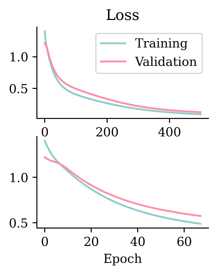
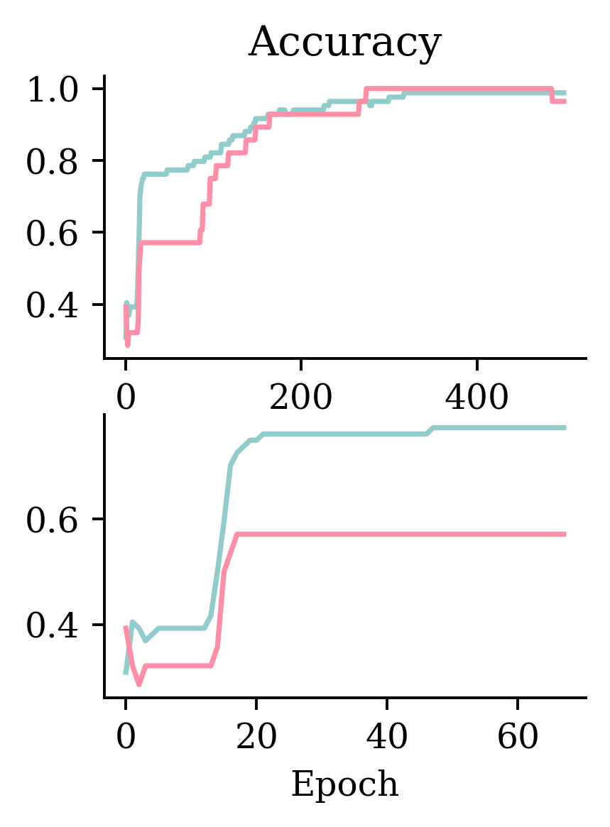
Left hand side plots show how loss behaved without and with early stopping. Right hand side plots show how accuracy performed without and with early stopping.

Add metrics, compile, and fit

model = create_model()

pr_auc = keras.metrics.AUC(curve="PR", name="pr_auc")
model.compile(optimizer="adam", loss="binary_crossentropy",
    metrics=[pr_auc, "accuracy", "auc"])                                

es = EarlyStopping(patience=50, restore_best_weights=True,
    monitor="val_pr_auc", verbose=1)
model.fit(X_train, y_train, callbacks=[es], epochs=1_000, verbose=0,
  validation_data=(X_val, y_val));

Epoch 65: early stopping
Restoring model weights from the end of the best epoch: 15.

1. Brings in the created model
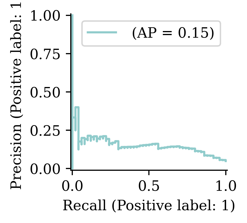
2. Creates an instance pr_auc to store the AUC (Area Under Curve) metric for the PR (Precision-Recall) curve
3. Compiles the model with an appropriate loss function, optimizer and relevant metrics. Since the above problem is a binary classification, we would optimize the binary_crossentropy, chose to monitor both accuracy and AUC and pr_auc.

Tracking AUC and pr_auc on top of the accuracy is important, particularly in the cases where there is a class imbalance. Suppose a data has 95% True class and only 5% False class, then, even a random classifier that predicts True 95% of the time will have a high accuracy. To avoid such issues, it is advisable to monitor both accuracy and AUC.

model.evaluate(X_val, y_val, verbose=0)

[0.14444081485271454,
 0.13122102618217468,
 0.9589040875434875,
 0.8215014934539795]

Cross-entropy loss: ELI5

Why use cross-entropy loss?

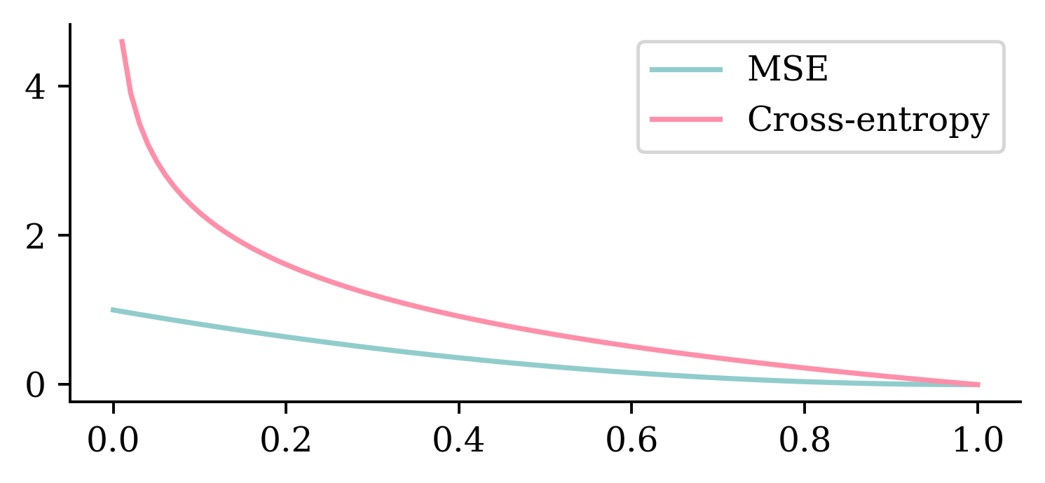
p = np.linspace(0, 1, 100)
plt.plot(p, (1 - p) ** 2)
plt.plot(p, -np.log(p))
plt.legend(["MSE", "Cross-entropy"]);

/var/folders/sc/b5vy9t2d2_scccwgx6kbk8w80000gp/T/ipykernel_17897/1829931169.py:3: RuntimeWarning: divide by zero encountered in log
  plt.plot(p, -np.log(p))

The above plot shows how MSE and cross-entropy penalize wrong predictions. The x-axis indicates the severity of misclassification. Suppose the neural network predicted that there is near-zero probability of an observation being in class “1” when the actual class is “1”. This represents a strong misclassification. The above graph shows how MSE does not impose heavy penalties for the misclassifications near zero. It displays a linear increment across the severity of misclassification. On the other hand, cross-entropy penalises bad predictions strongly. Also, the misclassification penalty grows exponentially. This makes cross entropy more suitable.

Overweight the minority class

model = create_model()

pr_auc = keras.metrics.AUC(curve="PR", name="pr_auc")
model.compile(optimizer="adam", loss="binary_crossentropy",
    metrics=[pr_auc, "accuracy", "auc"])

es = EarlyStopping(patience=50, restore_best_weights=True,
    monitor="val_pr_auc", verbose=1)
model.fit(X_train, y_train.to_numpy(), callbacks=[es], epochs=1_000, verbose=0,
  validation_data=(X_val, y_val), class_weight={0: 1, 1: 10});

Epoch 74: early stopping
Restoring model weights from the end of the best epoch: 24.

Another way to treat class imbalance would be to assign a higher weight to the minority class during model fitting. 1. Fits the model by assigning a higher weight to the misclassification in the minor class. This above class weight assignment says that misclassifying an observation from class 1 will be penalized 10 times more than misclassifying an observation from class 0. The weights can be assigned in relation to the level of data imbalance.

model.evaluate(X_val, y_val, verbose=0)

[0.3345569670200348,
 0.13615098595619202,
 0.8062622547149658,
 0.812220573425293]

model.evaluate(X_test, y_test, verbose=0)

[0.3590189516544342, 0.1449822038412094, 0.8023483157157898, 0.791563868522644]

Classification Metrics

from sklearn.metrics import confusion_matrix, RocCurveDisplay, PrecisionRecallDisplay
y_pred = model.predict(X_test, verbose=0)

RocCurveDisplay.from_predictions(y_test, y_pred, name="");

PrecisionRecallDisplay.from_predictions(y_test, y_pred, name=""); plt.legend(loc="upper right");

y_pred_stroke = y_pred > 0.5
confusion_matrix(y_test, y_pred_stroke)

array([[792, 180],
       [ 22,  28]])

y_pred_stroke = y_pred > 0.3
confusion_matrix(y_test, y_pred_stroke)

array([[662, 310],
       [ 10,  40]])

Example 2: Multiclass Classification

Iris dataset

from sklearn.datasets import load_iris
iris = load_iris()
names = ["SepalLength", "SepalWidth", "PetalLength", "PetalWidth"]
features = pd.DataFrame(iris.data, columns=names)
features

	SepalLength	SepalWidth	PetalLength	PetalWidth
0	5.1	3.5	1.4	0.2
1	4.9	3.0	1.4	0.2
...	...	...	...	...
148	6.2	3.4	5.4	2.3
149	5.9	3.0	5.1	1.8

150 rows × 4 columns

Target variable

iris.target_names

array(['setosa', 'versicolor', 'virginica'], dtype='<U10')

iris.target[:8]

array([0, 0, 0, 0, 0, 0, 0, 0])

target = iris.target
target = target.reshape(-1, 1)
target[:8]

array([[0],
       [0],
       [0],
       [0],
       [0],
       [0],
       [0],
       [0]])

classes, counts = np.unique(
        target,
        return_counts=True
)
print(classes)
print(counts)

[0 1 2]
[50 50 50]

iris.target_names[
  target[[0, 30, 60]]
]

array([['setosa'],
       ['setosa'],
       ['versicolor']], dtype='<U10')

Split the data into train and test

X_train, X_test, y_train, y_test = train_test_split(features, target, random_state=24)
X_train

	SepalLength	SepalWidth	PetalLength	PetalWidth
53	5.5	2.3	4.0	1.3
58	6.6	2.9	4.6	1.3
95	5.7	3.0	4.2	1.2
...	...	...	...	...
145	6.7	3.0	5.2	2.3
87	6.3	2.3	4.4	1.3
131	7.9	3.8	6.4	2.0

112 rows × 4 columns

X_test.shape, y_test.shape

((38, 4), (38, 1))

A basic classifier network

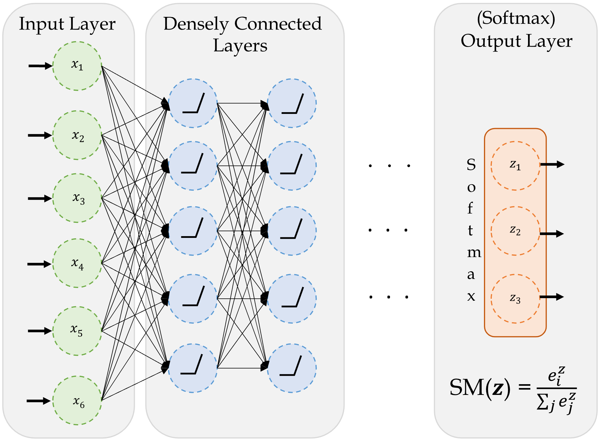
A basic network for classifying into three categories.

Source: Marcus Lautier (2022).

Since the task is a classification problem, we use softmax activation function. The softmax function takes in the input and returns a probability vector, which tells us about the probability of a data point belonging to a certain class.

Create a classifier model

NUM_FEATURES = len(features.columns)
NUM_CATS = len(np.unique(target))

print("Number of features:", NUM_FEATURES)
print("Number of categories:", NUM_CATS)

Number of features: 4
Number of categories: 3

Make a function to return a Keras model:

def build_model(seed=42):
    random.seed(seed)
    return Sequential([
        Dense(30, activation="relu"),
        Dense(NUM_CATS, activation="softmax")
    ])

Fit the model

model = build_model()
model.compile("adam", "sparse_categorical_crossentropy")

model.fit(X_train, y_train, epochs=5, verbose=2);

Epoch 1/5
4/4 - 0s - 66ms/step - loss: 1.3502
Epoch 2/5
4/4 - 0s - 5ms/step - loss: 1.2852
Epoch 3/5
4/4 - 0s - 5ms/step - loss: 1.2337
Epoch 4/5
4/4 - 0s - 5ms/step - loss: 1.1915
Epoch 5/5
4/4 - 0s - 5ms/step - loss: 1.1556

Since the problem at hand is a classification problem, we define the optimizer and loss function accordingly. Optimizer is adam and the loss function is sparse_categorical_crossentropy. If the response variable represents the category directly using an integer (i.e. if the response variable is not one-hot encoded), we must use sparse_categorical_crossentropy. If the response variable (y label) is already one-hot encoded we can use categorical_crossentropy.

Track accuracy as the model trains

model = build_model()
model.compile("adam", "sparse_categorical_crossentropy", metrics=["accuracy"])
model.fit(X_train, y_train, epochs=5, verbose=2);

Epoch 1/5
4/4 - 0s - 79ms/step - accuracy: 0.2946 - loss: 1.3502
Epoch 2/5
4/4 - 0s - 5ms/step - accuracy: 0.3036 - loss: 1.2852
Epoch 3/5
4/4 - 0s - 5ms/step - accuracy: 0.3036 - loss: 1.2337
Epoch 4/5
4/4 - 0s - 5ms/step - accuracy: 0.3304 - loss: 1.1915
Epoch 5/5
4/4 - 0s - 5ms/step - accuracy: 0.3393 - loss: 1.1556

We can also specify which loss metric to monitor in assessing the performance during the training. The metric that is usually used in classification tasks is accuracy, which tracks the fraction of all predictions which identified the class accurately. The metrics are not used for optimizing. They are only used to keep track of how well the model is performing during the optimization. By setting verbose=2, we are printing the progress during training, and we can see how the loss is reducing and accuracy is improving.

Run a long fit

Run the model training for 500 epochs.

model = build_model()
model.compile("adam", "sparse_categorical_crossentropy", \
        metrics=["accuracy"])
%time hist = model.fit(X_train, y_train, epochs=500, \
        validation_split=0.25, verbose=False)

CPU times: user 19.3 s, sys: 1.68 s, total: 21 s
Wall time: 19.3 s

Evaluation now returns both loss and accuracy.

model.evaluate(X_test, y_test, verbose=False)

[0.09586217254400253, 0.9736841917037964]

Add early stopping

model_es = build_model()
model_es.compile("adam", "sparse_categorical_crossentropy", \
        metrics=["accuracy"])

es = EarlyStopping(restore_best_weights=True, patience=50,
        monitor="val_accuracy")                                         
%time hist_es = model_es.fit(X_train, y_train, epochs=500, \
        validation_split=0.25, callbacks=[es], verbose=False);

print(f"Stopped after {len(hist_es.history['loss'])} epochs.")

CPU times: user 3.13 s, sys: 282 ms, total: 3.41 s
Wall time: 3.13 s
Stopped after 68 epochs.

1. Use build_model to make a new empty neural network to train
2. Compiles the model with optimizer, loss function and metric
3. Defines the early stopping object as usual, with one slight change. The code is specified to activate the early stopping by monitoring the validation accuracy (val_accuracy), not the loss.
4. Fits the model

Evaluation on test set:

model_es.evaluate(X_test, y_test, verbose=False)

[0.9856259226799011, 0.5263158082962036]

Fitting metrics

matplotlib.pyplot.rcParams["figure.figsize"] = (2.5, 2.95)
plt.subplot(2, 1, 1)
plt.plot(hist.history["loss"])
plt.plot(hist.history["val_loss"])
plt.title("Loss")
plt.legend(["Training", "Validation"])

plt.subplot(2, 1, 2)
plt.plot(hist_es.history["loss"])
plt.plot(hist_es.history["val_loss"])
plt.xlabel("Epoch");

matplotlib.pyplot.rcParams["figure.figsize"] = (2.5, 3.25)
plt.subplot(2, 1, 1)
plt.plot(hist.history["accuracy"])
plt.plot(hist.history["val_accuracy"])
plt.title("Accuracy")

plt.subplot(2, 1, 2)
plt.plot(hist_es.history["accuracy"])
plt.plot(hist_es.history["val_accuracy"])
plt.xlabel("Epoch");

Left hand side plots show how loss behaved without and with early stopping. Right hand side plots show how accuracy performed without and with early stopping.

What is the softmax activation?

It creates a “probability” vector: \text{Softmax}(\boldsymbol{x}) = \frac{\mathrm{e}^x_i}{\sum_j \mathrm{e}^x_j} \,.

In NumPy:

out = np.array([5, -1, 6])
(np.exp(out) / np.exp(out).sum()).round(3)

array([0.269, 0.001, 0.731])

In Keras:

out = keras.ops.convert_to_tensor([[5.0, -1.0, 6.0]])
keras.ops.round(keras.ops.softmax(out), 3)

<tf.Tensor: shape=(1, 3), dtype=float32, numpy=array([[0.269, 0.001, 0.731]], dtype=float32)>

Prediction using classifiers

y_test[:4]

array([[2],
       [2],
       [1],
       [1]])

The response variable y is an array of numeric integers, each representing a class to which the data belongs. However, the model.predict() function returns an array with probabilities not an array with integers. The array displays the probabilities of belonging to each category.

y_pred = model.predict(X_test.head(4), verbose=0)
y_pred

array([[4.9469954e-06, 8.1675522e-02, 9.1831952e-01],
       [4.1672743e-06, 7.0206067e-03, 9.9297523e-01],
       [9.2273308e-03, 9.7335482e-01, 1.7417978e-02],
       [3.1080188e-03, 8.7022400e-01, 1.2666793e-01]], dtype=float32)

Using np.argmax() which returns index of the maximum value in an array, we can obtain the predicted class.

# Add 'keepdims=True' to get a column vector.
np.argmax(y_pred, axis=1)

array([2, 2, 1, 1])

iris.target_names[np.argmax(y_pred, axis=1)]

array(['virginica', 'virginica', 'versicolor', 'versicolor'], dtype='<U10')

Summary

Classification models in Keras

If the target is a categorical variable with only two options, this is a binary classification problem. The neural network’s output layer should have one neuron with a sigmoid activation function. The loss function should be binary cross-entropy. In Keras, this is called loss="binary_crossentropy".

If the target has more than two options, this is a multi-class classification problem. The neural network’s output layer should have as many neurons as there are classes with a softmax activation function. The loss function should be categorical cross-entropy. In Keras, this is done with loss="sparse_categorical_crossentropy".

If the number of classes is c, then:

Target	Output Layer	Loss Function
Binary (c=2)	1 neuron with sigmoid activation	Binary Cross-Entropy
Multi-class (c > 2)	c neurons with softmax activation	Categorical Cross-Entropy

Optionally output logits

If you find that the training is unstable, you can try to use a linear activation in the final layer and have the loss functions implement the activation function.

If the number of classes is c, then:

Target	Output Layer	Loss Function
Binary (c=2)	1 neuron with linear activation	Binary Cross-Entropy (from_logits=True)
Multi-class (c > 2)	c neurons with linear activation	Categorical Cross-Entropy (from_logits=True)

Code examples

Binary

model = Sequential([
  # Skipping the earlier layers
  Dense(1, activation="sigmoid")
])
model.compile(loss="binary_crossentropy")

Multi-class

model = Sequential([
  # Skipping the earlier layers
  Dense(n_classes, activation="softmax")
])
model.compile(loss="sparse_categorical_crossentropy")

Binary (logits)

from keras.losses import BinaryCrossentropy
model = Sequential([
  # Skipping the earlier layers
  Dense(1, activation="linear")
])
loss = BinaryCrossentropy(from_logits=True)
model.compile(loss=loss)

Multi-class (logits)

from keras.losses import SparseCategoricalCrossentropy

model = Sequential([
  # Skipping the earlier layers
  Dense(n_classes, activation="linear")
])
loss = SparseCategoricalCrossentropy(from_logits=True)
model.compile(loss=loss)

Package Versions

from watermark import watermark
print(watermark(python=True, packages="keras,matplotlib,numpy,pandas,seaborn,scipy,torch,tensorflow,tf_keras"))

Python implementation: CPython
Python version       : 3.11.12
IPython version      : 9.3.0

keras     : 3.8.0
matplotlib: 3.10.0
numpy     : 2.0.2
pandas    : 2.2.2
seaborn   : 0.13.2
scipy     : 1.15.3
torch     : 2.6.0
tensorflow: 2.18.0
tf_keras  : 2.18.0

Glossary

• accuracy
• classification problem
• confusion matrix
• cross-entropy loss
• metrics
• sigmoid activation function
• softmax activation