Preprocessing

ACTL3143 & ACTL5111 Deep Learning for Actuaries

Author

Patrick Laub

Show the package imports

import random
from pathlib import Path

import matplotlib.pyplot as plt
import numpy as np
import pandas as pd

from keras.models import Sequential
from keras.layers import Dense, Input
from keras.callbacks import EarlyStopping

import sklearn
from sklearn.model_selection import train_test_split
from sklearn.preprocessing import OneHotEncoder, StandardScaler
from sklearn.impute import SimpleImputer
from sklearn.linear_model import LinearRegression

Deep learning project life cycle

Define objectives
Collect & label data
Clean & preprocess data (opt. feature engineering)
Design network architecture
Train and validate model
Hyperparameter tuning
Test and evaluate performance
Deploy to production
Monitor and iterate

(We won’t cover the italicised items in this course, though they are very important.)

Overview

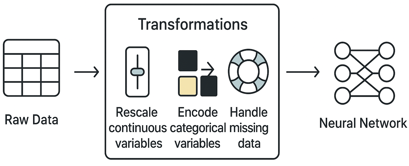
Every dataset needs to be transformed in various ways before it can be fed into a machine learning model.

Preprocessing refers to the transformations of the raw data before input to the network

Some steps are specific to neural networks (e.g. standardising continuous variables), others are necessary for every model (e.g. encoding categorical variables, handling missing data).

Example 1: Continuous Variables

California housing dataset

features, target = sklearn.datasets.fetch_california_housing(
    as_frame=True, return_X_y=True)
features

	MedInc	HouseAge	AveRooms	AveBedrms	Population	AveOccup	Latitude	Longitude
0	8.3252	41.0	6.984127	1.023810	322.0	2.555556	37.88	-122.23
1	8.3014	21.0	6.238137	0.971880	2401.0	2.109842	37.86	-122.22
...	...	...	...	...	...	...	...	...
20638	1.8672	18.0	5.329513	1.171920	741.0	2.123209	39.43	-121.32
20639	2.3886	16.0	5.254717	1.162264	1387.0	2.616981	39.37	-121.24

20640 rows × 8 columns

All the features were continuous variables

Can look at the data types of the features.

features.info()

<class 'pandas.core.frame.DataFrame'>
RangeIndex: 20640 entries, 0 to 20639
Data columns (total 8 columns):
 #   Column      Non-Null Count  Dtype  
---  ------      --------------  -----  
 0   MedInc      20640 non-null  float64
 1   HouseAge    20640 non-null  float64
 2   AveRooms    20640 non-null  float64
 3   AveBedrms   20640 non-null  float64
 4   Population  20640 non-null  float64
 5   AveOccup    20640 non-null  float64
 6   Latitude    20640 non-null  float64
 7   Longitude   20640 non-null  float64
dtypes: float64(8)
memory usage: 1.3 MB

Note that this isn’t foolproof. If you have ‘postcode’ as a feature, it may be read in as a number when it should be stored as a string and treated as a categorical variable.

Splitting into train, validation and test sets

X_main, X_test_raw, y_main, y_test = train_test_split(
    features, target, test_size=0.2, random_state=1
)
X_train_raw, X_val_raw, y_train, y_val = train_test_split(
    X_main, y_main, test_size=0.25, random_state=1
)

Note that we really cannot allow there to be duplicate rows in the training, validation, or test sets. If there are, we will have data leakage between the sets, which will lead to overfitting and poor generalisation.

Checking for leaks

We can look for rows that appear in multiple of the datasets.

train_val_overlap = pd.merge(X_train_raw, X_val_raw, how='inner')
train_test_overlap = pd.merge(X_train_raw, X_test_raw, how='inner')
val_test_overlap = pd.merge(X_val_raw, X_test_raw, how='inner')

print(f"Number of duplicated rows between train and val: {len(train_val_overlap)}")
print(f"Number of duplicated rows between train and test: {len(train_test_overlap)}")
print(f"Number of duplicated rows between val and test: {len(val_test_overlap)}")

Number of duplicated rows between train and val: 0
Number of duplicated rows between train and test: 0
Number of duplicated rows between val and test: 0

An earlier check is to check that there are no duplicate rows in the dataset.

features.duplicated().sum()

np.int64(0)

We rescaled every column

scaler = StandardScaler()
scaler.fit(X_train_raw)

X_train = scaler.transform(X_train_raw)
X_val = scaler.transform(X_val_raw)
X_test = scaler.transform(X_test_raw)

X_train

array([[ 0.15, -0.76,  0.26, ..., -0.01, -0.47,  0.69],
       [-1.79, -1.48,  0.48, ..., -0.08, -0.44,  1.33],
       [-0.97, -0.13, -0.67, ...,  0.05, -0.86,  0.65],
       ...,
       [ 0.11, -0.84, -0.54, ..., -0.03, -0.81,  0.6 ],
       [-0.82,  0.99, -0.03, ..., -0.03,  0.54, -0.11],
       [ 0.9 , -1.56,  0.66, ...,  0.07, -0.75,  0.97]])

That is because the neural network expects continuous inputs to be normalised to help with the training procedure.

Basically, the initial starting point for the network are random weights and biases that assume a (roughly) standard normal kind of input, to keep the inner neuron values from overflowing or underflowing.

Note

Notice that the output of X_train here looks a bit different to X_train_raw earlier? We’ll touch on this in a couple of slides.

Scikit-learn preprocessing methods

fit: learn the parameters of the transformation
transform: apply the transformation
fit_transform: learn the parameters and apply the transformation

fit
fit_transform

scaler = StandardScaler()
scaler.fit(X_train_raw)
X_train = scaler.transform(X_train_raw)
X_val = scaler.transform(X_val_raw)
X_test = scaler.transform(X_test_raw)

print(X_train.mean(axis=0))
print(X_train.std(axis=0))
print(X_val.mean(axis=0))
print(X_val.std(axis=0))

[ 1.11e-16 -1.08e-16 -2.81e-16  3.75e-16 -5.02e-18 -4.36e-17  1.15e-15
  1.75e-15]
[1. 1. 1. 1. 1. 1. 1. 1.]
[ 0.01  0.01  0.   -0.01 -0.    0.01  0.   -0.01]
[1.01 1.   0.81 0.81 0.98 0.84 0.99 1.  ]

scaler = StandardScaler()
X_train = scaler.fit_transform(X_train_raw)
X_val = scaler.transform(X_val_raw)
X_test = scaler.transform(X_test_raw)

print(X_train.mean(axis=0))
print(X_train.std(axis=0))
print(X_val.mean(axis=0))
print(X_val.std(axis=0))

[ 1.11e-16 -1.08e-16 -2.81e-16  3.75e-16 -5.02e-18 -4.36e-17  1.15e-15
  1.75e-15]
[1. 1. 1. 1. 1. 1. 1. 1.]
[ 0.01  0.01  0.   -0.01 -0.    0.01  0.   -0.01]
[1.01 1.   0.81 0.81 0.98 0.84 0.99 1.  ]

It is important to make sure that the scaler is fitted using only the data from the train set.

Dataframes & arrays

X_test_raw.head(3)

	MedInc	HouseAge	AveRooms	AveBedrms	Population	AveOccup	Latitude	Longitude
4712	3.2500	39.0	4.503205	1.073718	1109.0	1.777244	34.06	-118.36
2151	1.9784	37.0	4.988584	1.038813	1143.0	2.609589	36.78	-119.78
15927	4.0132	46.0	4.480296	1.012315	1534.0	3.778325	37.73	-122.42

X_test

array([[-0.33,  0.83, -0.34, ..., -0.11, -0.73,  0.6 ],
       [-1.  ,  0.67, -0.16, ..., -0.04,  0.54, -0.1 ],
       [ 0.07,  1.38, -0.35, ...,  0.06,  0.98, -1.42],
       ...,
       [ 0.62, -0.21, -0.16, ...,  0.05,  0.92, -1.4 ],
       [ 0.53,  1.07, -0.03, ..., -0.  , -0.72,  0.73],
       [-0.62,  1.86,  0.11, ..., -0.02, -0.77,  1.09]])

Note

By default, when you pass sklearn a DataFrame it returns a numpy array.

Keep as a DataFrame

From scikit-learn 1.2:

from sklearn import set_config
set_config(transform_output="pandas")

imp = SimpleImputer()

X_train = imp.fit_transform(X_train_raw)
X_val = imp.transform(X_val_raw)
X_test = imp.transform(X_test_raw)

Imports set_config function from sklearn.
Tells sklearn that any transformed data should stay as pandas dataframes.
Defines the SimpleImputer. This function helps in dealing with missing values. Default is set to mean, meaning that, missing values in each column will be replaced with the column mean.
Finds the means of training set columns, and replaces train set missing values by those means.
Replace missing values in the validation set by the means of the training set columns.
Replace missing values in the test set by the means of the training set columns.

From SimpleImputer’s docs:

X_test

	MedInc	HouseAge	AveRooms	AveBedrms	Population	AveOccup	Latitude	Longitude
4712	3.2500	39.0	4.503205	1.073718	1109.0	1.777244	34.06	-118.36
2151	1.9784	37.0	4.988584	1.038813	1143.0	2.609589	36.78	-119.78
...	...	...	...	...	...	...	...	...
6823	4.8750	42.0	5.347985	1.058608	829.0	3.036630	34.09	-118.10
11878	2.7054	52.0	5.741214	1.060703	905.0	2.891374	33.99	-117.38

4128 rows × 8 columns

Replace missing values using a descriptive statistic (e.g. mean, median, or most frequent) along each column, or using a constant value… default=‘mean’

Example 2: Continuous and Categorical Variables

French motor dataset

 # Download the dataset if we don't have it already. 
if not Path("french-motor.csv").exists():
    freq = sklearn.datasets.fetch_openml(data_id=41214, as_frame=True).frame
    freq.to_csv("french-motor.csv", index=False)
else:
    freq = pd.read_csv("french-motor.csv")
freq.info()

<class 'pandas.core.frame.DataFrame'>
RangeIndex: 678013 entries, 0 to 678012
Data columns (total 12 columns):
 #   Column      Non-Null Count   Dtype  
---  ------      --------------   -----  
 0   IDpol       678013 non-null  float64
 1   ClaimNb     678013 non-null  float64
 2   Exposure    678013 non-null  float64
 3   Area        678013 non-null  object 
 4   VehPower    678013 non-null  float64
 5   VehAge      678013 non-null  float64
 6   DrivAge     678013 non-null  float64
 7   BonusMalus  678013 non-null  float64
 8   VehBrand    678013 non-null  object 
 9   VehGas      678013 non-null  object 
 10  Density     678013 non-null  float64
 11  Region      678013 non-null  object 
dtypes: float64(8), object(4)
memory usage: 62.1+ MB

Checks if the dataset does not already exist within the current directory.
Download the dataset from sklearn. The fetch_openml function allows the user to bring in the datasets available in the OpenML platform. Every dataset has a unique ID, hence, can be fetched by providing the ID. data_id of the French motor dataset is 41214.
Save it as a CSV file, so we don’t need to redownload it (slow!) next time.
If it already exists, then read the dataset from the CSV file.

The data

freq

	IDpol	ClaimNb	Exposure	Area	VehPower	VehAge	DrivAge	BonusMalus	VehBrand	VehGas	Density	Region
0	1.0	1.0	0.10000	D	5.0	0.0	55.0	50.0	B12	Regular	1217.0	R82
1	3.0	1.0	0.77000	D	5.0	0.0	55.0	50.0	B12	Regular	1217.0	R82
2	5.0	1.0	0.75000	B	6.0	2.0	52.0	50.0	B12	Diesel	54.0	R22
...	...	...	...	...	...	...	...	...	...	...	...	...
678010	6114328.0	0.0	0.00274	D	6.0	2.0	45.0	50.0	B12	Diesel	1323.0	R82
678011	6114329.0	0.0	0.00274	B	4.0	0.0	60.0	50.0	B12	Regular	95.0	R26
678012	6114330.0	0.0	0.00274	B	7.0	6.0	29.0	54.0	B12	Diesel	65.0	R72

678013 rows × 12 columns

Data dictionary

IDpol: policy number (unique identifier)
ClaimNb: number of claims on the given policy
Exposure: total exposure in yearly units
Area: area code (categorical, ordinal)
VehPower: power of the car (categorical, ordinal)
VehAge: age of the car in years
DrivAge: age of the (most common) driver in years

BonusMalus: bonus-malus level between 50 and 230 (with reference level 100)
VehBrand: car brand (categorical, nominal)
VehGas: diesel or regular fuel car (binary)
Density: of inhabitants per km² in the city of the living place of the driver
Region: regions in France (prior to 2016)

We have \{ (\mathbf{x}_i, y_i) \}_{i=1, \dots, n} for \mathbf{x}_i \in \mathbb{R}^{p} and y_i \in \mathbb{N}_0. Assume the distribution Y_i \sim \mathsf{Poisson}(\lambda(\mathbf{x}_i))

We have \mathbb{E} Y_i = \lambda(\mathbf{x}_i). The NN takes \mathbf{x}_i & predicts \mathbb{E} Y_i.

freq = freq.drop("IDpol", axis=1)

Split the data

X_train_raw, X_test_raw, y_train, y_test = train_test_split(
  freq.drop("ClaimNb", axis=1), freq["ClaimNb"], random_state=2023)
X_train_raw = X_train_raw.reset_index(drop=True)
X_test_raw = X_test_raw.reset_index(drop=True)
X_train_raw

	Exposure	Area	VehPower	VehAge	DrivAge	BonusMalus	VehBrand	VehGas	Density	Region
0	0.01	A	4.0	0.0	70.0	50.0	B12	Regular	37.0	R72
1	1.00	C	6.0	11.0	36.0	50.0	B3	Regular	119.0	R82
2	0.08	D	7.0	9.0	35.0	50.0	B2	Diesel	1326.0	R93
...	...	...	...	...	...	...	...	...	...	...
508506	0.22	E	7.0	21.0	32.0	90.0	B5	Regular	4128.0	R52
508507	1.00	C	7.0	15.0	51.0	50.0	B1	Regular	461.0	R53
508508	0.42	D	6.0	1.0	37.0	54.0	B2	Diesel	1284.0	R25

508509 rows × 10 columns

Splits the dataset into train and test sets. By setting the random_state to a specific number, we ensure the consistency in the train-test split. freq.drop("ClaimNb", axis=1) removes the “ClaimNb” column.
Resets the index of train set, and drops the previous index column. Since the index column will get shuffled during the train-test split, we may want to reset the index to start from 0 again.

What values do we see in the data?

X_train_raw["Area"].value_counts()
X_train_raw["VehBrand"].value_counts()
X_train_raw["VehGas"].value_counts()
X_train_raw["Region"].value_counts()

Area
C    144156
D    113532
E    102791
A     78017
B     56571
F     13442
Name: count, dtype: int64

VehBrand
B12    124490
B1     122200
B2     120155
        ...  
B11     10218
B13      9160
B14      2998
Name: count, Length: 11, dtype: int64

VehGas
Regular    259422
Diesel     249087
Name: count, dtype: int64

Region
R24    120597
R82     63555
R93     59627
        ...  
R21      2283
R42      1634
R43      1024
Name: count, Length: 22, dtype: int64

data["column_name"].value_counts() function provides counts of each category for a categorical variable. In this dataset, variables Area and VehGas are assumed to have natural orderings whereas VehBrand and Region are not considered to have such natural orderings. Therefore, the two sets of categorical variables will have to be treated differently.

Nominal categorical variables

These are categorical variables which you cannot order in a ‘default’ sensible way.

from sklearn.preprocessing import OneHotEncoder
gas = X_train_raw[["VehGas"]]

The original data:

gas.head()

	VehGas
0	Regular
1	Regular
2	Diesel
3	Regular
4	Diesel

One-hot encoding

enc = OneHotEncoder(sparse_output=False)

X_train = enc.fit_transform(gas)
X_train.head()

	VehGas_Diesel	VehGas_Regular
0	0.0	1.0
1	0.0	1.0
2	1.0	0.0
3	0.0	1.0
4	1.0	0.0

Dummy encoding

enc = OneHotEncoder(
    drop="first",
    sparse_output=False)
X_train = enc.fit_transform(gas)
X_train.head()

	VehGas_Regular
0	1.0
1	1.0
2	0.0
3	1.0
4	0.0

Warning

Collinearity is not a big deal for neural networks. However if you want to reuse the same X_train data for a (generalised) linear regression, then you probably want to dummy-encode here to avoid needing two different preprocessing regimes for the two competing models.

Ordinal categorical variables

These are categorical variables which have a natural order to them.

from sklearn.preprocessing import OrdinalEncoder
enc = OrdinalEncoder()
enc.fit(X_train_raw[["Area"]])
enc.categories_

[array(['A', 'B', 'C', 'D', 'E', 'F'], dtype=object)]

OrdinalEncoder can assign numerical values to each category of the ordinal variable. The nice thing about OrdinalEncoder is that it can preserve the information about ordinal relationships in the data. To actually convert the values in the ordinal columns, we must also apply the enc.transform method. The following lines of code show how we consistently apply the transform function to both train and test sets. To avoid inconsistencies in encoding, we use enc.fit function only to the train set.

Imports the OrdinalEncoder from sklearn.preprocessing library
Create an OrdinalEncoder object named enc
Selects the two columns with ordinal variables from X_train and fits the ordinal encoder
Gives out the number of unique categories in each ordinal variable

for i, area in enumerate(enc.categories_[0]):
    print(f"The Area value {area} gets turned into {i}.")

The Area value A gets turned into 0.
The Area value B gets turned into 1.
The Area value C gets turned into 2.
The Area value D gets turned into 3.
The Area value E gets turned into 4.
The Area value F gets turned into 5.

In other words,

print(" < ".join(enc.categories_[0]) + ", and ")
print(" = ".join(f"{r} - {l}" for l, r in zip(enc.categories_[0][:-1], enc.categories_[0][1:])))

A < B < C < D < E < F, and 
B - A = C - B = D - C = E - D = F - E

Ordinal encoded values

Note that fitting an ordinal encoder (enc.fit) only establishes the mapping between numerical values and ordinal variable levels. To actually convert the values in the ordinal columns, we must also apply the enc.transform function. Following lines of code shows how we consistently apply the transform function to both train and test sets. To avoid inconsistencies in encoding, we use enc.fit function only to the train set.

X_train = enc.transform(X_train_raw[["Area"]])
X_test = enc.transform(X_test_raw[["Area"]])

X_train_raw[["Area"]].head()

	Area
0	A
1	C
2	D
3	E
4	B

X_train.head()

	Area
0	0.0
1	2.0
2	3.0
3	4.0
4	1.0

We could train on this X_train, or on the previous X_train, but each only contains one feature from the dataset. How do we add the continuous variables back in? Use a sklearn column transformer for that.

Transform each column in one hit

from sklearn.compose import make_column_transformer

ct = make_column_transformer(
  (OneHotEncoder(sparse_output=False, drop="first"), ["VehGas", "VehBrand", "Region"]),
  (OrdinalEncoder(), ["Area"]),
  remainder=StandardScaler()
)

X_train = ct.fit_transform(X_train_raw)

Imports the make_column_transformer class that can carry out data preparation selectively
Starts defining the column transformer object
Apply dummy encoding to the nominal categorical columns
Apply ordinal encoding to the ordinal categorical column
Standardise the remaining columns (which are all numerical)
Fits and transforms the train set using this new column transformer

X_train_raw

	Exposure	Area	VehPower	VehAge	DrivAge	BonusMalus	VehBrand	VehGas	Density	Region
0	0.01	A	4.0	0.0	70.0	50.0	B12	Regular	37.0	R72
...	...	...	...	...	...	...	...	...	...	...
508508	0.42	D	6.0	1.0	37.0	54.0	B2	Diesel	1284.0	R25

508509 rows × 10 columns

X_train

	onehotencoder__VehGas_Regular	onehotencoder__VehBrand_B10	onehotencoder__VehBrand_B11	onehotencoder__VehBrand_B12	onehotencoder__VehBrand_B13	onehotencoder__VehBrand_B14	onehotencoder__VehBrand_B2	onehotencoder__VehBrand_B3	onehotencoder__VehBrand_B4	onehotencoder__VehBrand_B5	...	onehotencoder__Region_R91	onehotencoder__Region_R93	onehotencoder__Region_R94	ordinalencoder__Area	remainder__Exposure	remainder__VehPower	remainder__VehAge	remainder__DrivAge	remainder__BonusMalus	remainder__Density
0	1.0	0.0	0.0	1.0	0.0	0.0	0.0	0.0	0.0	0.0	...	0.0	0.0	0.0	0.0	-1.424715	-1.196660	-1.245210	1.732277	-0.623438	-0.442987
...	...	...	...	...	...	...	...	...	...	...	...	...	...	...	...	...	...	...	...	...	...
508508	0.0	0.0	0.0	0.0	0.0	0.0	1.0	0.0	0.0	0.0	...	0.0	0.0	0.0	3.0	-0.299951	-0.221191	-1.068474	-0.602450	-0.367372	-0.127782

508509 rows × 39 columns

The default column names of X_train that the column transformer adds are a bit obscure/verbose. We can add the verbose_feature_names_out=False flag to have a cleaner X_train dataframe.

Transform each column in one hit II

from sklearn.compose import make_column_transformer

ct = make_column_transformer(
  (OneHotEncoder(sparse_output=False, drop="first"), ["VehGas", "VehBrand", "Region"]),
  (OrdinalEncoder(), ["Area"]),
  ("drop", ["VehBrand", "Region"]),
  remainder=StandardScaler(),
  verbose_feature_names_out=False
)
X_train = ct.fit_transform(X_train_raw)

X_train_raw

	Exposure	Area	VehPower	VehAge	DrivAge	BonusMalus	VehBrand	VehGas	Density	Region
0	0.01	A	4.0	0.0	70.0	50.0	B12	Regular	37.0	R72
...	...	...	...	...	...	...	...	...	...	...
508508	0.42	D	6.0	1.0	37.0	54.0	B2	Diesel	1284.0	R25

508509 rows × 10 columns

X_train

	VehGas_Regular	VehBrand_B10	VehBrand_B11	VehBrand_B12	VehBrand_B13	VehBrand_B14	VehBrand_B2	VehBrand_B3	VehBrand_B4	VehBrand_B5	...	Region_R91	Region_R93	Region_R94	Area	Exposure	VehPower	VehAge	DrivAge	BonusMalus	Density
0	1.0	0.0	0.0	1.0	0.0	0.0	0.0	0.0	0.0	0.0	...	0.0	0.0	0.0	0.0	-1.424715	-1.196660	-1.245210	1.732277	-0.623438	-0.442987
...	...	...	...	...	...	...	...	...	...	...	...	...	...	...	...	...	...	...	...	...	...
508508	0.0	0.0	0.0	0.0	0.0	0.0	1.0	0.0	0.0	0.0	...	0.0	0.0	0.0	3.0	-0.299951	-0.221191	-1.068474	-0.602450	-0.367372	-0.127782

508509 rows × 39 columns

An important thing to notice here is that, the order of columns have changed. They are rearranged according to the order in which we specify the transformations inside the column transformer.

Aside: The order of the variables matters

X_train_raw["Area_In_Words"] = X_train_raw["Area"].map({
    "A": "Very low", "B": "Low", "C": "Medium",
    "D": "High", "E": "Very high", "F": "Extremely high"
})

enc_wrong = OrdinalEncoder()
enc_wrong.fit(X_train_raw[["Area_In_Words"]])
enc_wrong.categories_

[array(['Extremely high', 'High', 'Low', 'Medium', 'Very high', 'Very low'],
       dtype=object)]

for i, area in enumerate(enc_wrong.categories_[0]):
    print(f"The Area value {area} gets turned into {i}.")

The Area value Extremely high gets turned into 0.
The Area value High gets turned into 1.
The Area value Low gets turned into 2.
The Area value Medium gets turned into 3.
The Area value Very high gets turned into 4.
The Area value Very low gets turned into 5.

In other words,

print(" < ".join(enc_wrong.categories_[0]))

Extremely high < High < Low < Medium < Very high < Very low

Aside: Manually set the order

ordered = [["Very low", "Low", "Medium", "High", "Very high", "Extremely high"]]
enc_right = OrdinalEncoder(categories=ordered)
enc_right.fit(X_train_raw[["Area_In_Words"]])
enc_right.categories_

[array(['Very low', 'Low', 'Medium', 'High', 'Very high', 'Extremely high'],
       dtype=object)]

for i, area in enumerate(enc_right.categories_[0]):
    print(f"The Area value {area} gets turned into {i}.")

The Area value Very low gets turned into 0.
The Area value Low gets turned into 1.
The Area value Medium gets turned into 2.
The Area value High gets turned into 3.
The Area value Very high gets turned into 4.
The Area value Extremely high gets turned into 5.

In other words,

print(" < ".join(enc_right.categories_[0]))

Very low < Low < Medium < High < Very high < Extremely high

X_train_raw = X_train_raw.drop("Area_In_Words", axis=1)

Example 3: Continuous and Categorical Variables and Missing Values

Stroke prediction dataset

Dataset source: Kaggle Stroke Prediction Dataset.

RAW_DATA_DIR = Path("stroke/raw")
data = pd.read_csv(RAW_DATA_DIR / "stroke.csv")
data.head()

	id	gender	age	hypertension	heart_disease	ever_married	work_type	Residence_type	avg_glucose_level	bmi	smoking_status	stroke
0	9046	Male	67.0	0	1	Yes	Private	Urban	228.69	36.6	formerly smoked	1
1	51676	Female	61.0	0	0	Yes	Self-employed	Rural	202.21	NaN	never smoked	1
2	31112	Male	80.0	0	1	Yes	Private	Rural	105.92	32.5	never smoked	1
3	60182	Female	49.0	0	0	Yes	Private	Urban	171.23	34.4	smokes	1
4	1665	Female	79.0	1	0	Yes	Self-employed	Rural	174.12	24.0	never smoked	1

Data description

id: unique identifier
gender: “Male”, “Female” or “Other”
age: age of the patient
hypertension: 0 or 1 if the patient has hypertension
heart_disease: 0 or 1 if the patient has any heart disease
ever_married: “No” or “Yes”
work_type: “children”, “Govt_job”, “Never_worked”, “Private” or “Self-employed”

Residence_type: “Rural” or “Urban”
avg_glucose_level: average glucose level in blood
bmi: body mass index
smoking_status: “formerly smoked”, “never smoked”, “smokes” or “Unknown”
stroke: 0 or 1 if the patient had a stroke

Look for missing values and split the data

First, look for missing values.

number_missing = data.isna().sum()
number_missing[number_missing > 0]

bmi    201
dtype: int64

Tip

Always take a look at the missing data in, say, Excel. Sometimes pandas reads in a category like “None” and interprets that as a missing value, when it’s really a valid category. This happened to me just the other day.

features = data.drop(["id", "stroke"], axis=1)
target = data["stroke"]

X_main_raw, X_test_raw, y_main, y_test = train_test_split(
    features, target, test_size=0.2, random_state=7)
X_train_raw, X_val_raw, y_train, y_val = train_test_split(
    X_main_raw, y_main, test_size=0.25, random_state=12)

X_train_raw.shape, X_val_raw.shape, X_test_raw.shape

((3066, 10), (1022, 10), (1022, 10))

What values do we see in the data?

X_train_raw["gender"].value_counts()

gender
Female    1802
Male      1264
Name: count, dtype: int64

X_train_raw["ever_married"].value_counts()

ever_married
Yes    2007
No     1059
Name: count, dtype: int64

X_train_raw["Residence_type"].value_counts()

Residence_type
Urban    1536
Rural    1530
Name: count, dtype: int64

X_train_raw["work_type"].value_counts()

work_type
Private          1754
Self-employed     490
children          419
Govt_job          390
Never_worked       13
Name: count, dtype: int64

X_train_raw["smoking_status"].value_counts()

smoking_status
never smoked       1130
Unknown             944
formerly smoked     522
smokes              470
Name: count, dtype: int64

Tip

Look for sparse categories. One common trick is to lump together all the small categories (e.g. < 5% or 10% each) into a new combined ‘OTHER’ or ‘RARE’ category.

Make a plan for preprocessing each column

Take categorical columns \hookrightarrow one-hot vectors
binary columns \hookrightarrow do nothing (already 0 & 1)
continuous columns \hookrightarrow impute NaNs & standardise.

Make the column transformer

from sklearn.pipeline import make_pipeline

nom_vars =  ["gender", "ever_married", "Residence_type",
    "work_type", "smoking_status"]                  

ct = make_column_transformer(
  (OneHotEncoder(sparse_output=False, handle_unknown="ignore"), nom_vars),
  ("passthrough", ["hypertension", "heart_disease"]),
  remainder=make_pipeline(SimpleImputer(), StandardScaler()),
  verbose_feature_names_out=False
)

X_train = ct.fit_transform(X_train_raw)
X_val = ct.transform(X_val_raw)
X_test = ct.transform(X_test_raw)

for name, X in zip(("train", "val", "test"), (X_train, X_val, X_test)):
    num_na = pd.DataFrame(X).isna().sum().sum()
    print(f"The {name} set has shape {X.shape} & with {num_na} NAs.")

The train set has shape (3066, 20) & with 0 NAs.
The val set has shape (1022, 20) & with 0 NAs.
The test set has shape (1022, 20) & with 0 NAs.

Imports make_pipeline class from sklearn.pipeline library. make_pipeline is used to streamline the data pre processing. In the above example, make_pipeline is used to first treat for missing values and then scale numerical values
Stores categorical variables in nom_vars
Specifies the one-hot encoding for all categorical variables. We set the sparse_output=False, to return a dense array rather than a sparse matrix. handle_unknown specifies how the neural network should handle unseen categories. By setting handle_unknown="ignore", we instruct the neural network to ignore categories that were not seen during training. If we did not do this, it will interrupt the model’s operation after deployment
Passes through hypertension and heart_disease without any pre processing
Makes a pipeline that first applies SimpleImputer() to replace missing values with the mean and then applies StandardScaler() to scale the numerical values
Prints out the missing values to ensure the SimpleImputer() has worked

Handling unseen categories

X_train_raw["gender"].value_counts()

gender
Female    1802
Male      1264
Name: count, dtype: int64

X_val_raw["gender"].value_counts()

gender
Female    615
Male      406
Other       1
Name: count, dtype: int64

Because the way train and test was split, one-hot encoder could not pick up on the third category. This could interrupt the model performance. To avoid such confusions, we could either give instructions manually on how to tackle unseen categories. An example is given below.

ind = np.argmax(X_val_raw["gender"] == "Other")
X_val_raw.iloc[ind-1:ind+3][["gender"]]

	gender
4970	Male
3116	Other
4140	Male
2505	Female

gender_cols = pd.DataFrame(X_val)[["gender_Female", "gender_Male"]]
gender_cols.iloc[ind-1:ind+3]

	gender_Female	gender_Male
4970	0.0	1.0
3116	0.0	0.0
4140	0.0	1.0
2505	1.0	0.0

However, to give such instructions on handling unseen categories, we would first have to know what those possible categories could be. We should also have specific knowledge on what value to assign in case they come up during model performance. One easy way to tackle it would be to use handle_unknown="ignore" during encoding, as mentioned before.

Handling unseen categories II

This was caused by fitting the encoder on the X_train which, by bad luck, didn’t have the “Other” category. Why not just read the entire dataset before splitting to collect all the values the categorical variables could take?

It’s a very mild form of data leakage, though it may be justifiable in some cases. If we made the datasets, we’d have a better idea of whether it makes sense on a case-by-case basis. We struggle here as we (in this course) are just analysing datasets which we didn’t collect.

Save the preprocessed data to files

PROCESSED_DATA_DIR = Path("stroke/processed")
PROCESSED_DATA_DIR.mkdir(parents=True, exist_ok=True)

X_train.to_csv(PROCESSED_DATA_DIR / "x_train.csv", index=False)
X_val.to_csv(PROCESSED_DATA_DIR / "x_val.csv", index=False)
X_test.to_csv(PROCESSED_DATA_DIR / "x_test.csv", index=False)
y_train.to_csv(PROCESSED_DATA_DIR / "y_train.csv", index=False)
y_val.to_csv(PROCESSED_DATA_DIR / "y_val.csv", index=False)
y_test.to_csv(PROCESSED_DATA_DIR / "y_test.csv", index=False)

Lastly, keep the preprocessor around

Later want to make a prediction on some new data point. It has to go through the exact same preprocessing steps.

import joblib
joblib.dump(ct, PROCESSED_DATA_DIR / "preprocessor.pkl")
preprocessor = joblib.load(PROCESSED_DATA_DIR / "preprocessor.pkl")

X_test_raw.head(1)

	gender	age	hypertension	heart_disease	ever_married	work_type	Residence_type	avg_glucose_level	bmi	smoking_status
2804	Female	69.0	0	0	Yes	Govt_job	Rural	70.98	30.0	Unknown

new_data = X_test_raw.head(1).copy()
new_data["ever_married"] = "No" # Let's pretend this is the new data point

ct.transform(new_data)

	gender_Female	gender_Male	ever_married_No	ever_married_Yes	Residence_type_Rural	Residence_type_Urban	work_type_Govt_job	work_type_Never_worked	work_type_Private	work_type_Self-employed	work_type_children	smoking_status_Unknown	smoking_status_formerly smoked	smoking_status_never smoked	smoking_status_smokes	hypertension	heart_disease	age	avg_glucose_level	bmi
2804	1.0	0.0	1.0	0.0	1.0	0.0	1.0	0.0	0.0	0.0	0.0	1.0	0.0	0.0	0.0	0	0	1.154917	-0.778758	0.147508

preprocessor.transform(new_data)

	gender_Female	gender_Male	ever_married_No	ever_married_Yes	Residence_type_Rural	Residence_type_Urban	work_type_Govt_job	work_type_Never_worked	work_type_Private	work_type_Self-employed	work_type_children	smoking_status_Unknown	smoking_status_formerly smoked	smoking_status_never smoked	smoking_status_smokes	hypertension	heart_disease	age	avg_glucose_level	bmi
2804	1.0	0.0	1.0	0.0	1.0	0.0	1.0	0.0	0.0	0.0	0.0	1.0	0.0	0.0	0.0	0	0	1.154917	-0.778758	0.147508

Glossary

column transformer
nominal variables
ordinal variables
one-hot encoding
missing values
imputation
standardisation