Bonus–malus level between 50 and 230 (with reference level 100)
Normalised
VehBrand*
Car brand (nominal)
One-hot
VehGas
Diesel or regular fuel car (binary)
One-hot
Density
Density of inhabitants per km2 in the city of the living place of the driver
Normalised
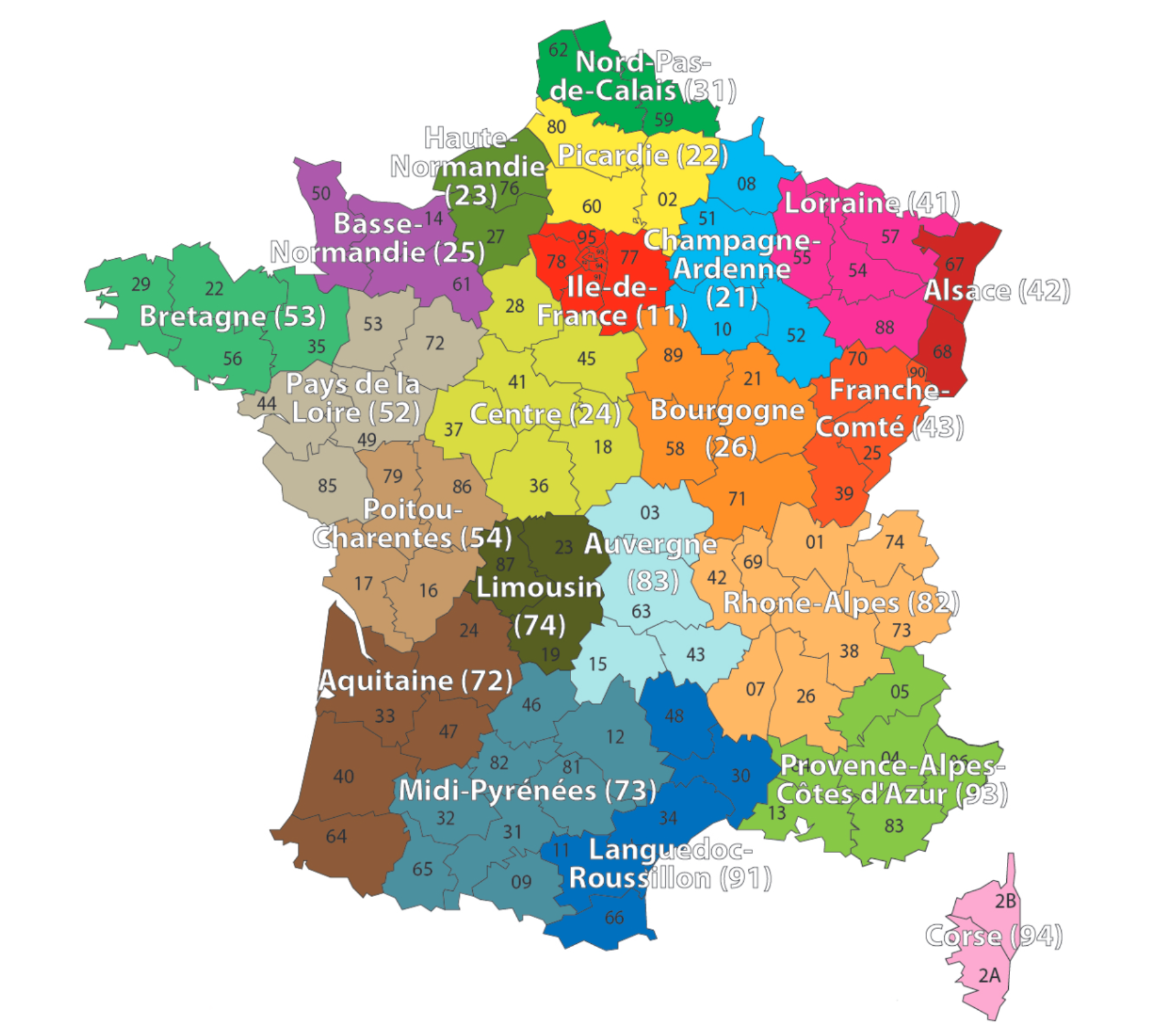
Region*
Regions in France (prior to 2016)
One-hot
The model
Have \{ (\mathbf{x}_i, y_i) \}_{i=1, \dots, n} for \mathbf{x}_i \in \mathbb{R}^{47} and y_i \in \mathbb{N}_0.
Assume the distribution
Y_i \sim \mathsf{Poisson}(\lambda(\mathbf{x}_i))
We have \mathbb{E} Y_i = \lambda(\mathbf{x}_i). The NN takes \mathbf{x}_i & predicts \mathbb{E} Y_i.
Note
For insurance, this is a bit weird. The exposures are different for each policy.
\lambda(\mathbf{x}_i) is the expected number of claims for the duration of policy i’s contract.
Normally, \text{Exposure}_i \not\in \mathbf{x}_i, and \lambda(\mathbf{x}_i) is the expected rate per year, then
Y_i \sim \mathsf{Poisson}(\text{Exposure}_i \times \lambda(\mathbf{x}_i)).
What values do we see in the data?
Code
freq = freq.drop("IDpol", axis=1).head(25_000)X_train, X_test, y_train, y_test = train_test_split( freq.drop("ClaimNb", axis=1), freq["ClaimNb"], random_state=36861)# Reset each index to start at 0 again.X_train_raw = X_train.reset_index(drop=True)X_test_raw = X_test.reset_index(drop=True)
One hot encoding is a way to assign numerical values to nominal variables. One hot encoding is different from ordinal encoding in the way in which it transforms the data. Ordinal encoding assigns a numerical integer to each unique category of the data column and returns one integer column. In contrast, one hot encoding returns a binary vector for each unique category. As a result, what we get from one hot encoding is not a single column vector, but a matrix with number of columns equal to the number of unique categories in that nominal data column.
Computes the number of unique categories in the encoded column and store it in num_regions
2
Constructs the neural network. This time, it is a neural network with 1 hidden layer and 1 output layer. Dense(2, input_dim=num_regions) takes in an input matrix with columns = num_regions and transforms it down to an output with 2 neurons
3
Steps 3-6 are similar to what we saw during training with ordinal encoded variables
/Users/z3535837/DeepLearningForActuaries/.venv/lib/python3.13/site-packages/keras/src/layers/core/dense.py:93: UserWarning:

Do not pass an `input_shape`/`input_dim` argument to a layer. When using Sequential models, prefer using an `Input(shape)` object as the first layer in the model instead.
Epoch 6: early stopping
0.7679625153541565
Make a fake batch of data
Make a fake batch of data where one observation is from each region (essentially an identity matrix). We use this fake batch of data to see what the hidden layer’s activation looks like under each of the 22 categories.
X = np.eye(num_regions)pd.DataFrame(X, columns=oh.categories_[0])
The above codes manually compute and return the same answers as before. Remember that our \mathbf X is the identity matrix, so any matrix multiplication with \mathbf X becomes redundant (X @ W + b == W + b). This is extremely valuable as, if your categorical variable had, say, 10,000 different category possibilities, the matrix operation becomes intensive.
Just a look-up operation
We can consider this as just a look-up operation, where each row of the matrix W+b is some vector representation of each category. For example, if we want to know how region 11 is represented, we just look at the first row of the matrix W+b.
To use the entity embedding functionality, we need to turn the categories into indices. We can use the oridinal encoder to do so.
oe = OrdinalEncoder()X_train_reg = oe.fit_transform(X_train_raw[["Region"]])X_test_reg = oe.transform(X_test_raw[["Region"]])for i, reg inenumerate(oe.categories_[0][:3]):print(f"The Region value {reg} gets turned into {i}.")
The Region value R11 gets turned into 0.
The Region value R21 gets turned into 1.
The Region value R22 gets turned into 2.
Use an Embedding layer
Feed this new version of the data into the NN, using an embedding layer.
Embedding layer can learn the optimal representation for a category of a categorical variable, during training. In the above example, encoding the variable Region using ordinal encoding and passing it through an embedding layer learns the optimal representation for the region during training. Ordinal encoding followed with an embedding layer is a better alternative to one-hot encoding. It is computationally less expensive (compared to generating large matrices in one-hot encoding) particularly when the number of categories is high.
The regions in get converted from text to index to vector representation in the embedding layer for each observation.
Entity embedding is especially useful when there is a very large number of categories (such as 1,000 or 10,000) and you want to reduce the number of columns. If your categorical variable has n categories, a simple rule of thumb is to use n^{1/4} for the dimension of the entity embedding.
In this case, the dimension chosen was 2. The intuition behind this is that regions can be represented easily over a 2-dimensional plane (by their geographical coordinates).
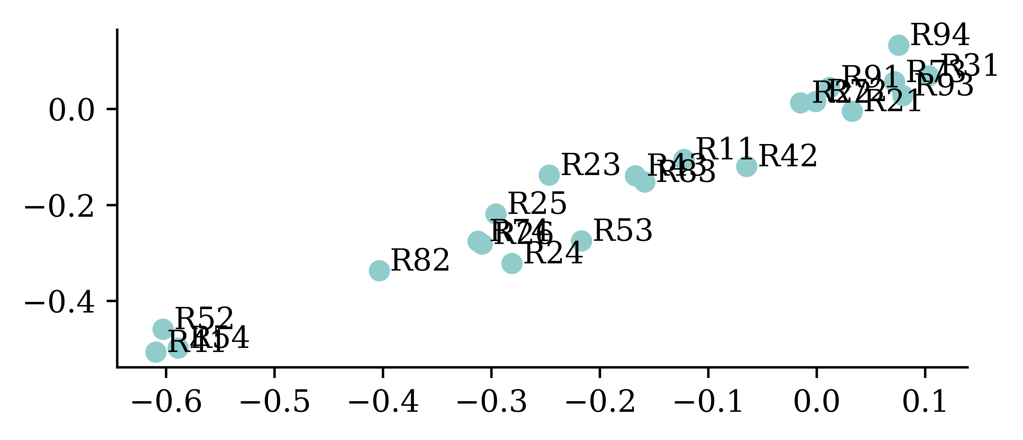
The learned embeddings
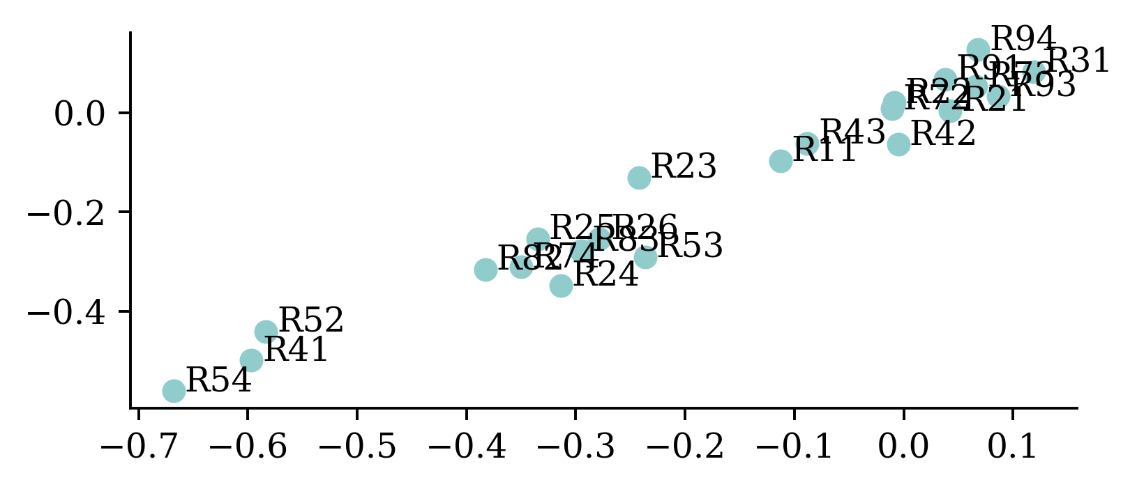
If we only have two-dimensional embeddings we can plot them.
points = model.layers[0].get_weights()[0]plt.scatter(points[:,0], points[:,1])for i inrange(num_regions): plt.text(points[i,0]+0.01, points[i,1] , s=oe.categories_[0][i])
While it not always the case, entity embeddings can at times be meaningful instead of just being useful representations. The above figure shows how plotting the learned embeddings help reveal regions which might be similar (e.g. coastal areas, hilly areas etc.).
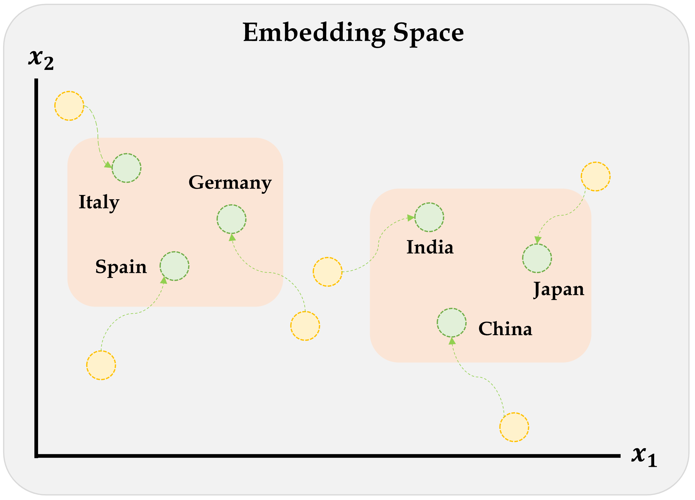
Entity embeddings
Embeddings will gradually improve during training.
Each category is initially assigned a random vector, but they move during training. These movements follow some sort of logic, for example in this graph countries in Europe cluster together and countries in Asia cluster together.
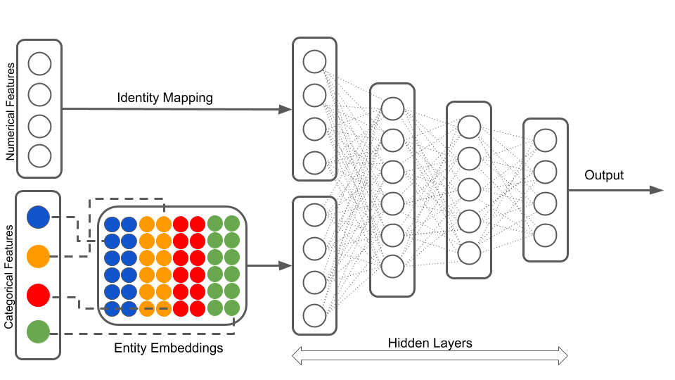
Embeddings & other inputs
Often times, we deal with both categorical and numerical variables together. The following diagram shows a recommended way of inputting numerical and categorical data in to the neural network. Numerical variables are inherently numeric and do not require entity embedding. On the other hand, categorical variables must undergo entity embedding to convert to number format.
Illustration of a neural network with both continuous and categorical inputs.
We can’t do this with Sequential models…
Given we want numerical variables to do one thing and categorical variables to do another, they need to be preprocessed separately and independently. The outputs of these independent (non-sequential) preprocesses become inputs to the next hidden layer (now back to sequential).
Keras’ Functional API
Sequential models are easy to use and do not require many specifications, however, they cannot model complex neural network architectures. Keras Functional API approach on the other hand allows the users to build complex architectures.
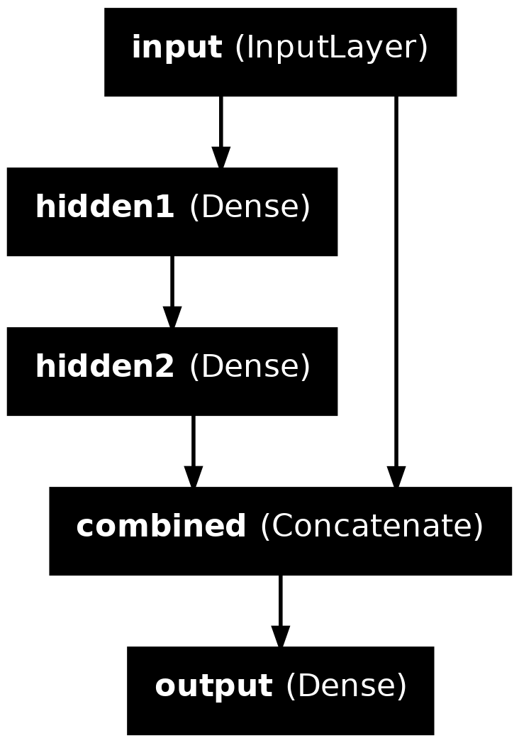
Converting Sequential models
from keras.models import Modelfrom keras.layers import Input
The above code shows how to construct the same neural network using sequential models and Keras functional API. Every sequential model can be converted into the functional style, but not every functional model can be converted to the sequential style.
In the functional API approach, we must specify the shape of the input layer, and explicitly define the inputs and outputs of a layer before specifying the model. model = Model(inputs, out) specifies the inputs and outputs of the model. This manner of specifying the inputs and outputs of the model allows the user to combine several inputs (inputs which are preprocessed in different ways) to finally build the model. One example would be combining entity embedded categorical variables, and scaled numerical variables.
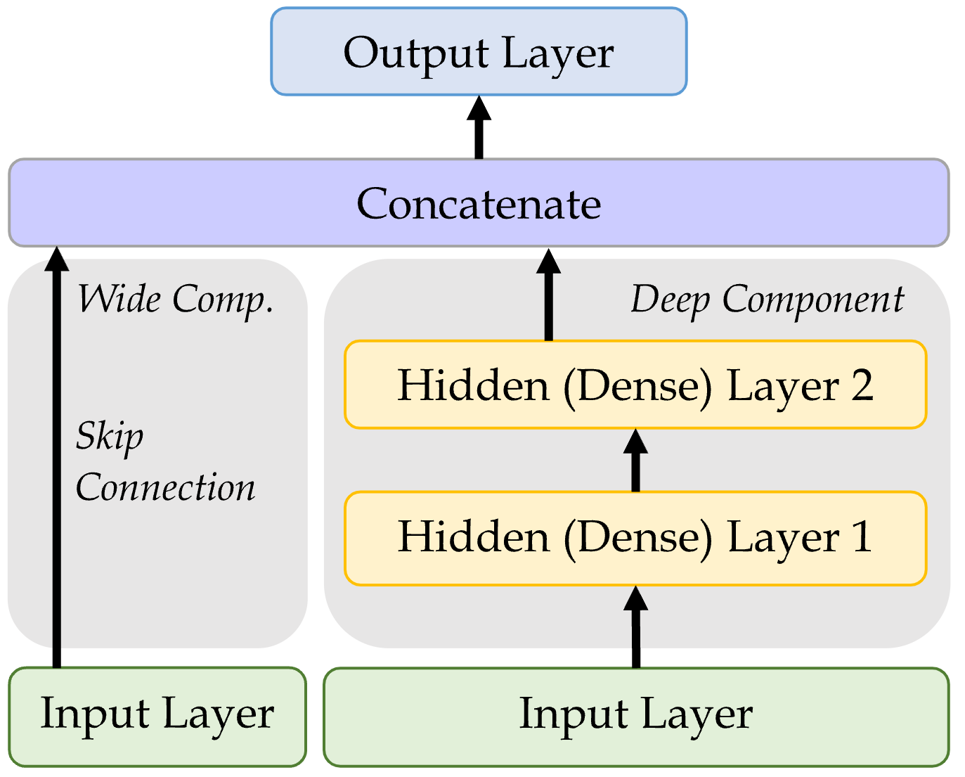
Wide & Deep network
An illustration of the wide & deep network architecture.
Add a skip connection from input to output layers.
The functional API method can unlock some new non-sequential NN architectures, such as the Wide & Deep network. One version of the inputs is processed through dense hidden layers, and the other version skips the processing. The two versions are then concatenated into a new layer which is used to create the output layer.
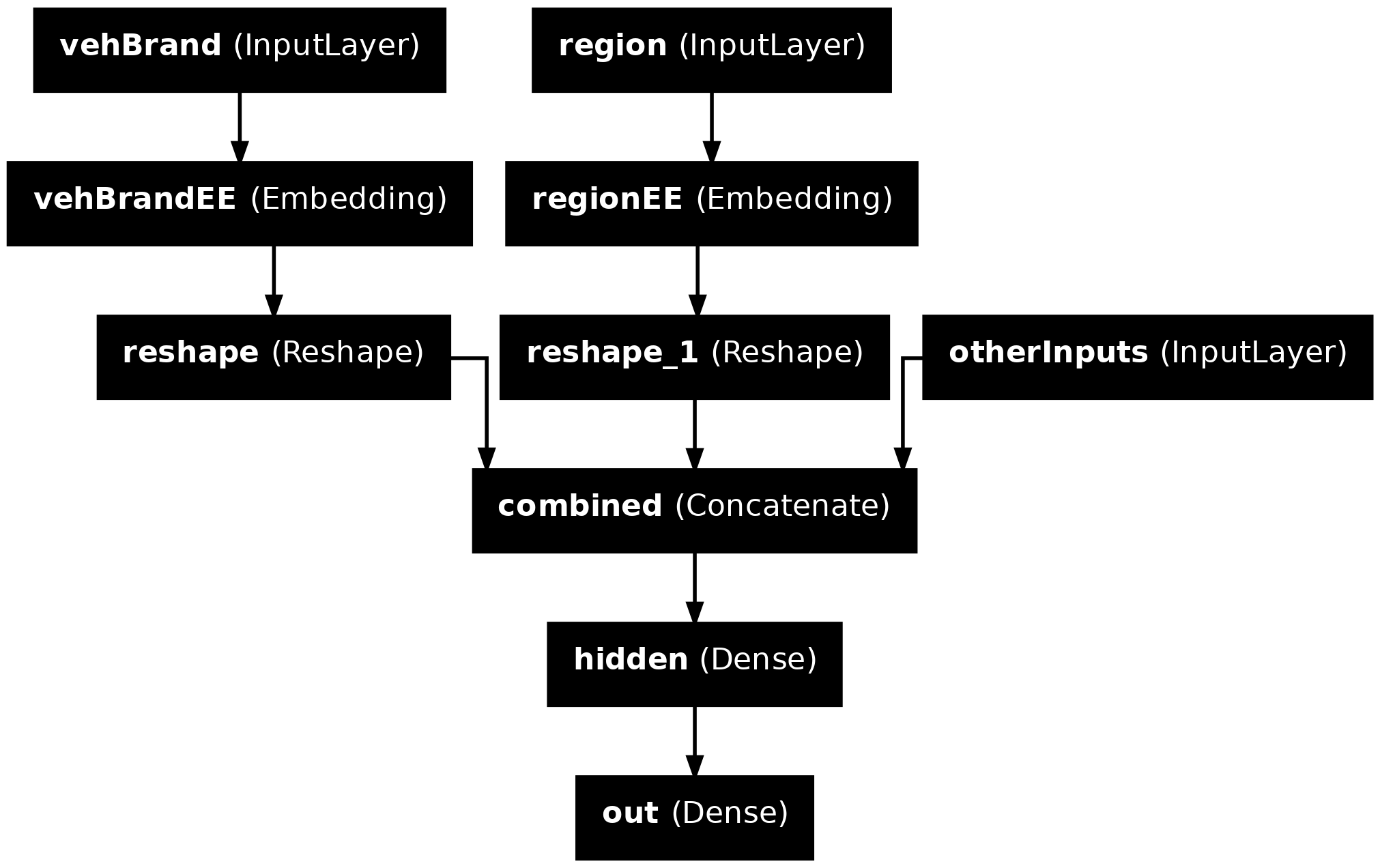
Naming the layers
For complex networks, it is often useful to give meaningful names to the layers.
Stores separately the number of unique categorical in the nominal variables, as would require these values later for entity embedding
2
Contructs columns transformer by first ordinally encoding all categorical variables (ordinal and nominal). Nominal variables are ordinal encoded here just as an intermediate step before this is the required input format for entity embedding layers
3
Applies standard scaling to all other numerical variables
4
Choose the simpler style of column names for the transformed dataframes
5
Fits the column transformer to the train set and transforms it
6
Transforms the test set using the column transformer fitted using the train set
Split the brand and region data apart from the rest:
Constructs the embedding layer by specifying the input dimension (the number of unique categories) and output dimension (the number of dimensions we want the input to be summarised in to)
3
Reshapes the output to match the format required at the model building step
4
Constructs the embedding layer by specifying the input dimension (the number of unique categories) and output dimension
5
Reshapes the output to match the format required at the model building step
6
Combines the entity embedded matrices and other inputs together
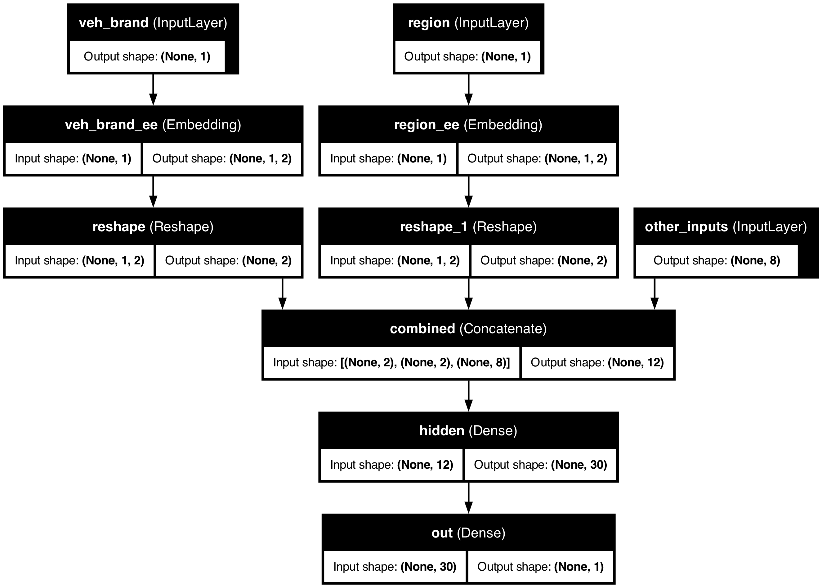
Complete the model and fit it
Feed the combined embeddings & continuous inputs to some normal dense layers.
The plotted model shows how, for example, region starts off as a matrix with (None,1) shape. This indicates that region was a column matrix with some number of rows. Entity embedding the region variable resulted in a 3D array of shape ((None,1,2)) which is not the required format for concatenating. Therefore, we reshape it using the Reshape function. This results in column array of shape, (None,2) which is what we need for concatenating.
Scale By Exposure
Two different models
Have \{ (\mathbf{x}_i, y_i) \}_{i=1, \dots, n} for \mathbf{x}_i \in \mathbb{R}^{47} and y_i \in \mathbb{N}_0.
Model 1: Say Y_i \sim \mathsf{Poisson}(\lambda(\mathbf{x}_i)).
But, the exposures are different for each policy. \lambda(\mathbf{x}_i) is the expected number of claims for the duration of policy i’s contract.
Model 2: Say Y_i \sim \mathsf{Poisson}(\text{Exposure}_i \times \lambda(\mathbf{x}_i)).
Now, \text{Exposure}_i \not\in \mathbf{x}_i, and \lambda(\mathbf{x}_i) is the rate per year.
Just take continuous variables
For convenience, the following code only considers the numerical variables during this implementation.