Optimisation

ACTL3143 & ACTL5111 Deep Learning for Actuaries

Author

Patrick Laub

Show the package imports

import random
import matplotlib.pyplot as plt
import numpy as np
import pandas as pd

Dense Layers in Matrices

Logistic regression

If we want to solve a binary classification problem, we can fit a logistic regression. We could say that a logistic regression is a neural network with no hidden layers and 1 neuron. z_i is a linear combination of the covariates for observation i. The activation function is \sigma(\cdot) which converts the z_i to a value y_i between 0 and 1, representing the probability of a positive outcome. The sigmoid activation function is the inverse logit function.

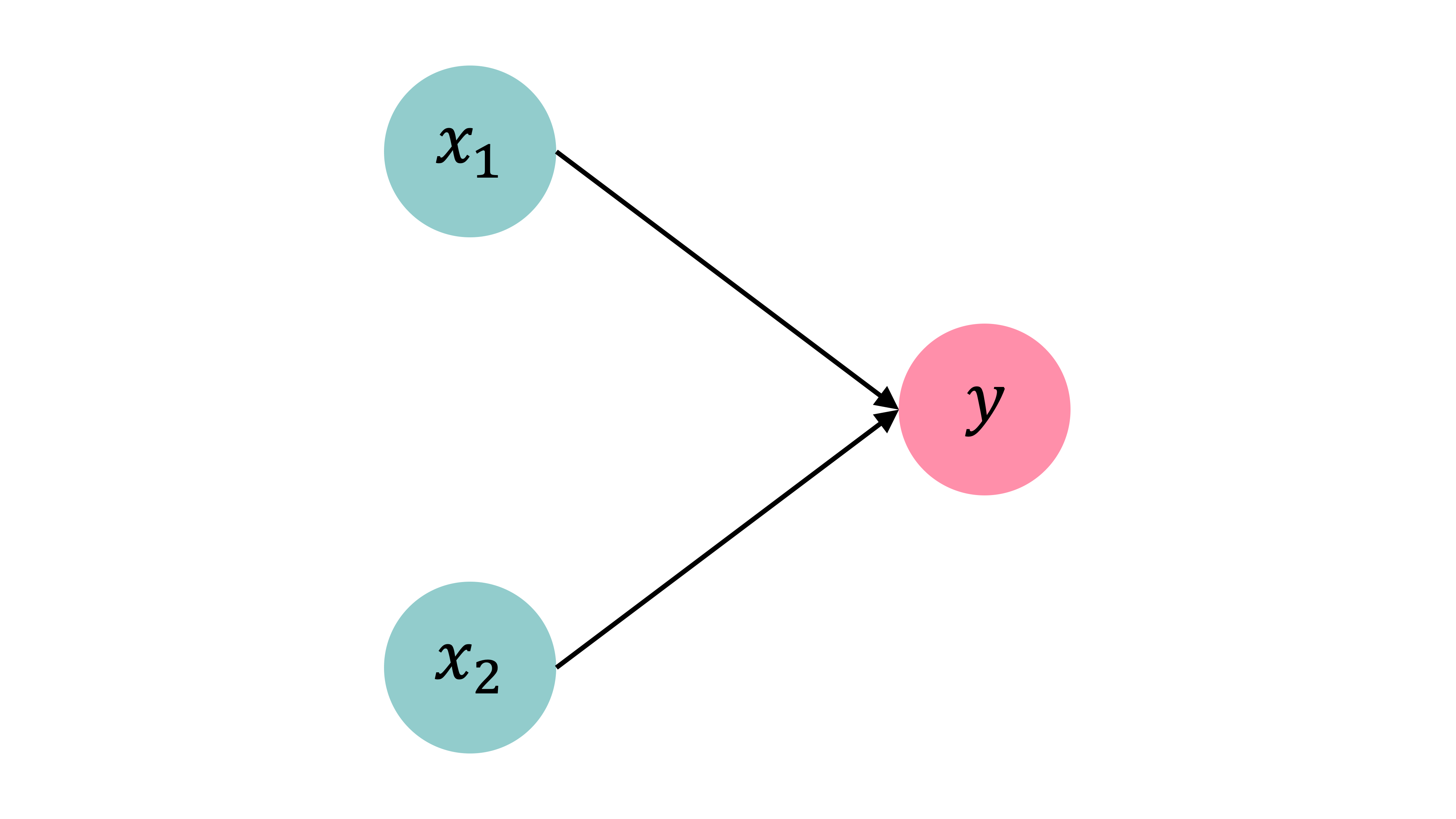
Observations: \mathbf{x}_{i,\bullet} \in \mathbb{R}^{2}.

Target: y_i \in \{0, 1\}.

Predict: \hat{y}_i = \mathbb{P}(Y_i = 1).

The model

For \mathbf{x}_{i,\bullet} = (x_{i,1}, x_{i,2}): z_i = x_{i,1} w_1 + x_{i,2} w_2 + b

\hat{y}_i = \sigma(z_i) = \frac{1}{1 + \mathrm{e}^{-z_i}} .

x = np.linspace(-10, 10, 100)
y = 1/(1 + np.exp(-x))
plt.plot(x, y);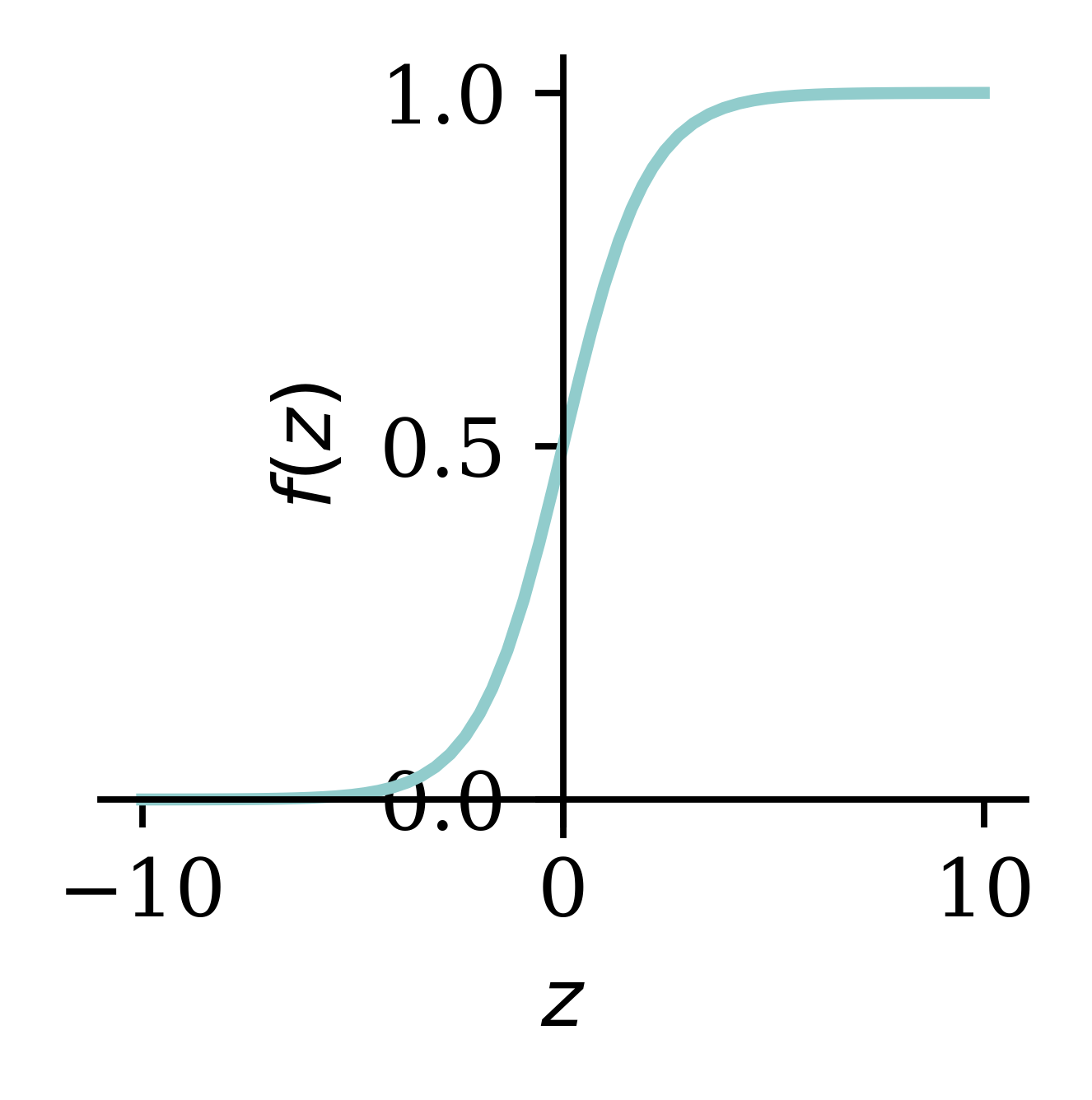

Multiple observations

When we have multiple observations, we can manually calculate the predicted values using the fitted weights and biases.

data = pd.DataFrame({"x_1": [1, 3, 5], "x_2": [2, 4, 6], "y": [0, 1, 1]})
data

	x_1	x_2	y
0	1	2	0
1	3	4	1
2	5	6	1

Let w_1 = 1, w_2 = 2 and b = -10.

w_1 = 1; w_2 = 2; b = -10
data["x_1"] * w_1 + data["x_2"] * w_2 + b

0   -5
1    1
2    7
dtype: int64

Matrix notation

Now let’s consider this in matrix notation. \mathbf{X} is the matrix of covariates, \mathbf{w} is the column vector of weights, b is a constant and \mathbf{z} is the output column vector before activation. Finally, \mathbf{a} is the output column vector after applying the activation function. Note that:

\text{number of columns in }\mathbf{X} = \text{number of rows in }\mathbf{w}
\text{number of rows in }\mathbf{X} = \text{number of rows in }\mathbf{z}
\text{number of rows in }\mathbf{z} = \text{number of rows in }\mathbf{a}

Have \mathbf{X} \in \mathbb{R}^{3 \times 2}.

X_df = data[["x_1", "x_2"]]
X = X_df.to_numpy()
X

array([[1, 2],
       [3, 4],
       [5, 6]])

Let \mathbf{w} = (w_1, w_2)^\top \in \mathbb{R}^{2 \times 1}.

w = np.array([[1], [2]])
w

array([[1],
       [2]])

\mathbf{z} = \mathbf{X} \mathbf{w} + b , \quad \mathbf{a} = \sigma(\mathbf{z})

z = X.dot(w) + b
z

array([[-5],
       [ 1],
       [ 7]])

1 / (1 + np.exp(-z))

array([[0.01],
       [0.73],
       [1.  ]])

Using a softmax output

This time, our problem is still a logistic regression problem, but with a softmax output. There are 2 neurons, each representing the probability that the target is in either category. In the context of matrices, this means that the output is a vector rather than a single value. Separate weights and biases are fitted for each neuron. The activation function is no longer sigmoid, but softmax. The predictions are converted to probability distributions.

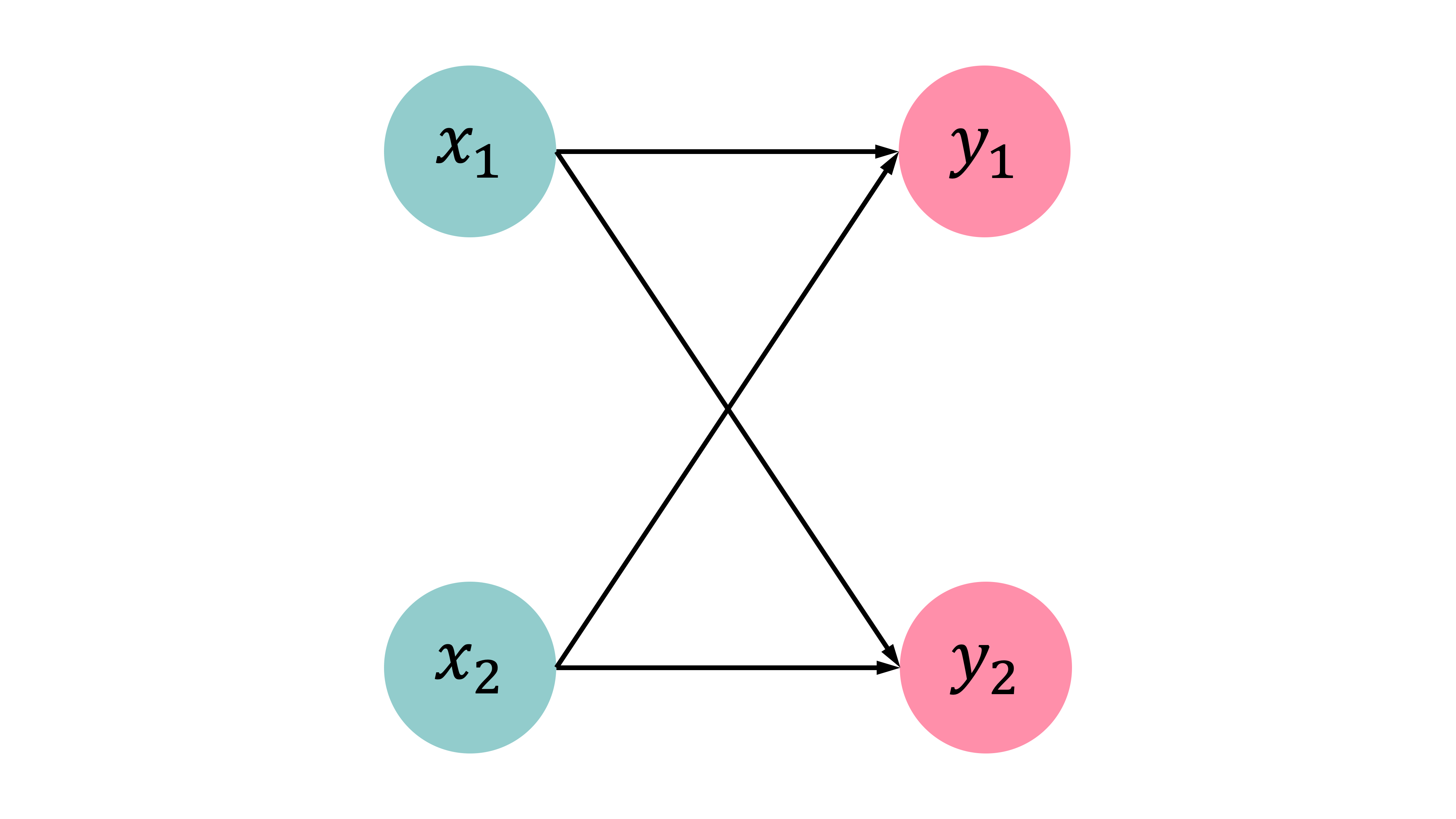
Observations: \mathbf{x}_{i,\bullet} \in \mathbb{R}^{2}. Predict: \hat{y}_{i,j} = \mathbb{P}(Y_i = j).

Target: \mathbf{y}_{i,\bullet} \in \{(1, 0), (0, 1)\}.

The model: For \mathbf{x}_{i,\bullet} = (x_{i,1}, x_{i,2}) \begin{aligned} z_{i,1} &= x_{i,1} w_{1,1} + x_{i,2} w_{2,1} + b_1 , \\ z_{i,2} &= x_{i,1} w_{1,2} + x_{i,2} w_{2,2} + b_2 . \end{aligned}

\begin{aligned} \hat{y}_{i,1} &= \text{Softmax}_1(\mathbf{z}_i) = \frac{\mathrm{e}^{z_{i,1}}}{\mathrm{e}^{z_{i,1}} + \mathrm{e}^{z_{i,2}}} , \\ \hat{y}_{i,2} &= \text{Softmax}_2(\mathbf{z}_i) = \frac{\mathrm{e}^{z_{i,2}}}{\mathrm{e}^{z_{i,1}} + \mathrm{e}^{z_{i,2}}} . \end{aligned}

Multiple observations

data

	x_1	x_2	y_1	y_2
0	1	2	1	0
1	3	4	0	1
2	5	6	0	1

Choose:

w_{1,1} = 1, w_{2,1} = 2,

w_{1,2} = 3, w_{2,2} = 4, and

b_1 = -10, b_2 = -20.

w_11 = 1; w_21 = 2; b_1 = -10
w_12 = 3; w_22 = 4; b_2 = -20
data["x_1"] * w_11 + data["x_2"] * w_21 + b_1

0   -5
1    1
2    7
dtype: int64

Matrix notation

Have \mathbf{X} \in \mathbb{R}^{3 \times 2}.

array([[1, 2],
       [3, 4],
       [5, 6]])

\mathbf{W}\in \mathbb{R}^{2\times2}, \mathbf{b}\in \mathbb{R}^{2}

W = np.array([[1, 3], [2, 4]])
b = np.array([-10, -20])
display(W); b

array([[1, 3],
       [2, 4]])

array([-10, -20])

\mathbf{Z} = \mathbf{X} \mathbf{W} + \mathbf{b} , \quad \mathbf{A} = \text{Softmax}(\mathbf{Z}) .

Z = X @ W + b
Z

array([[-5, -9],
       [ 1,  5],
       [ 7, 19]])

np.exp(Z) / np.sum(np.exp(Z),
  axis=1, keepdims=True)

array([[9.82e-01, 1.80e-02],
       [1.80e-02, 9.82e-01],
       [6.14e-06, 1.00e+00]])

Optimisation

Gradient-based learning

In-class demo

Gradient descent pitfalls

Depending on where the algorithm starts, it might find a local minimum, but not the global minimum.
If it starts where the gradient is very small, it may take a long time to get to the minimum because it will take small steps
If it starts where the gradient is 0 (plateau), the algorithm will have nowhere to go and end there.

Go over all the training data

Called batch gradient descent.

for i in range(num_epochs):
    gradient = evaluate_gradient(loss_function, data, weights)
    weights = weights - learning_rate * gradient

Batch gradient descent tries to improve all of the predictions in one go by using the entire training set at once.

For each epoch of the data, evaluate the gradient of the loss function on the entire training set with the chosen weights. The new weights are rebalanced based on the learning rate and in the negative direction of the gradient.

Pick a random training example

Called stochastic gradient descent.

for i in range(num_epochs):
    rnd.shuffle(data)
    for example in data:
        gradient = evaluate_gradient(loss_function, example, weights)
        weights = weights - learning_rate * gradient

Rather than trying to improve all predictions at once, stochastic gradient descent tries to improve each observation one by one (chosen at random). The weights are adjusted many times in a single epoch.

Take a group of training examples

Called mini-batch gradient descent.

for i in range(num_epochs):
    rnd.shuffle(data)
    for b in range(num_batches):
        batch = data[b * batch_size : (b + 1) * batch_size]
        gradient = evaluate_gradient(loss_function, batch, weights)
        weights = weights - learning_rate * gradient

Somewhere in between batch gradient descent and stochastic gradient descent, mini-batch gradient descent tries to improve batches of the training data at a time. The weights are adjusted a few times in a single epoch.

This is the most common method.

Mini-batch gradient descent

Most NNs opt for mini-batch gradient descent.

Why?

Because we have to (data is too big to shove it all in a single batch)
Because it is faster (lots of quick noisy steps takes longer than a few slow super accurate steps)
The noise helps us jump out of local minima

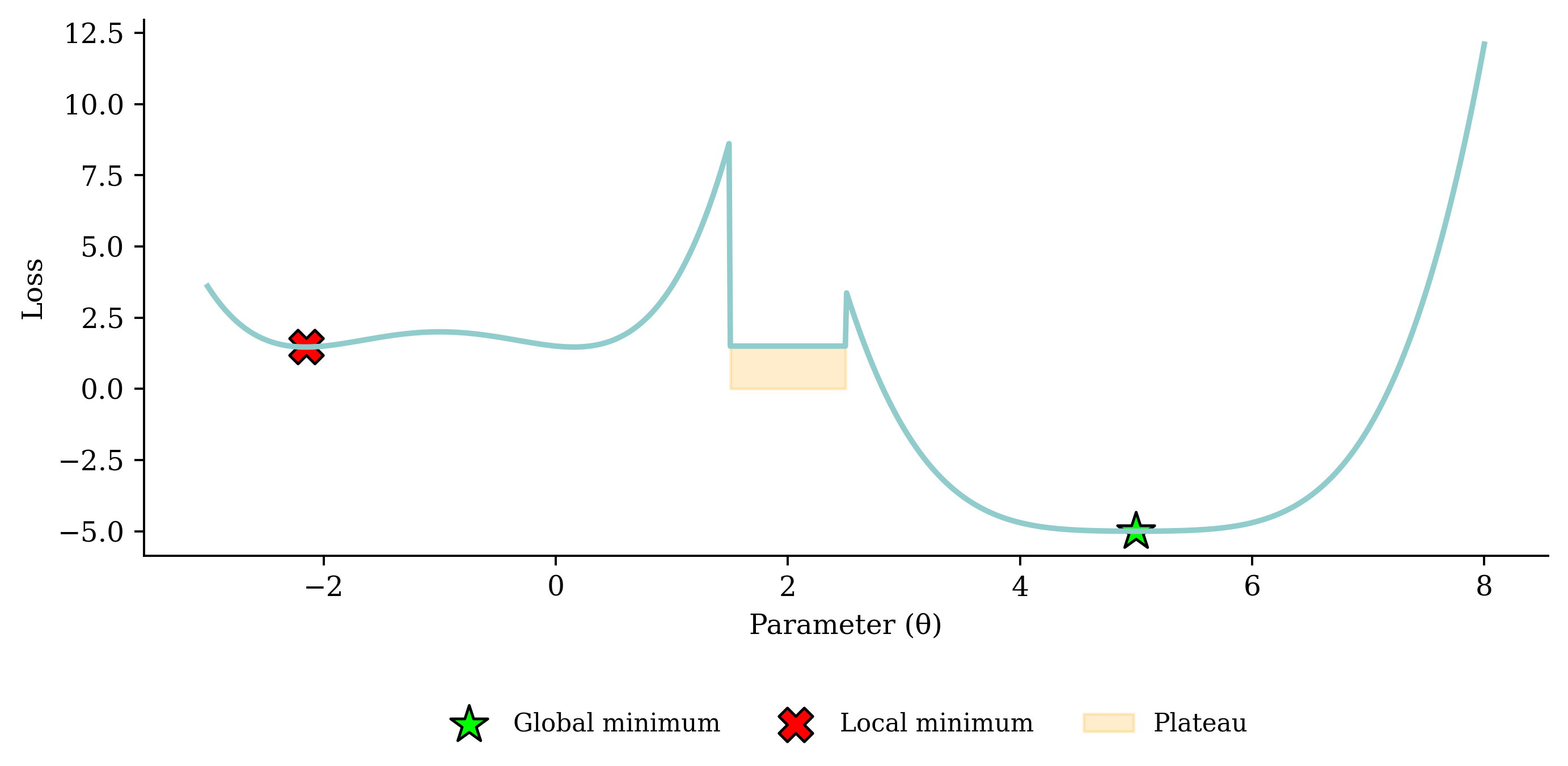
Noisy gradient means we might jump out of a local minimum.

Learning rates

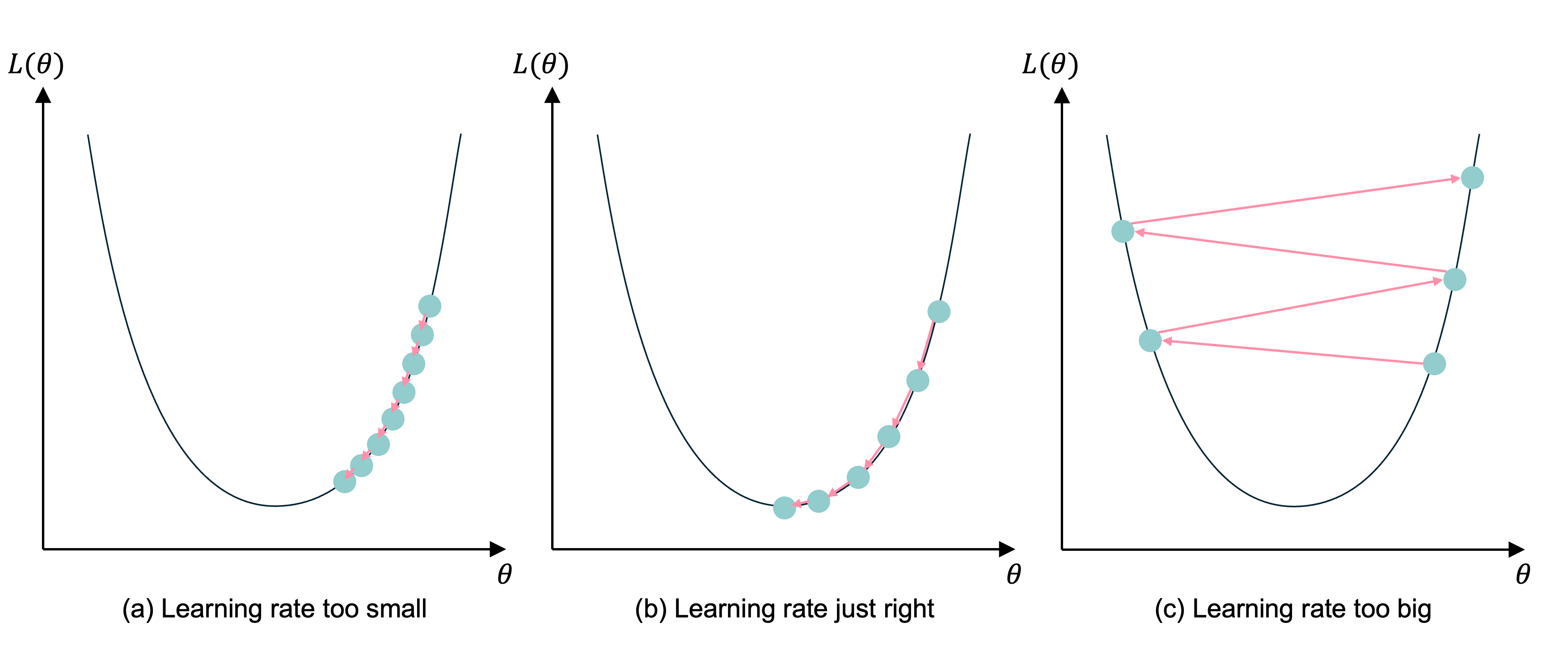
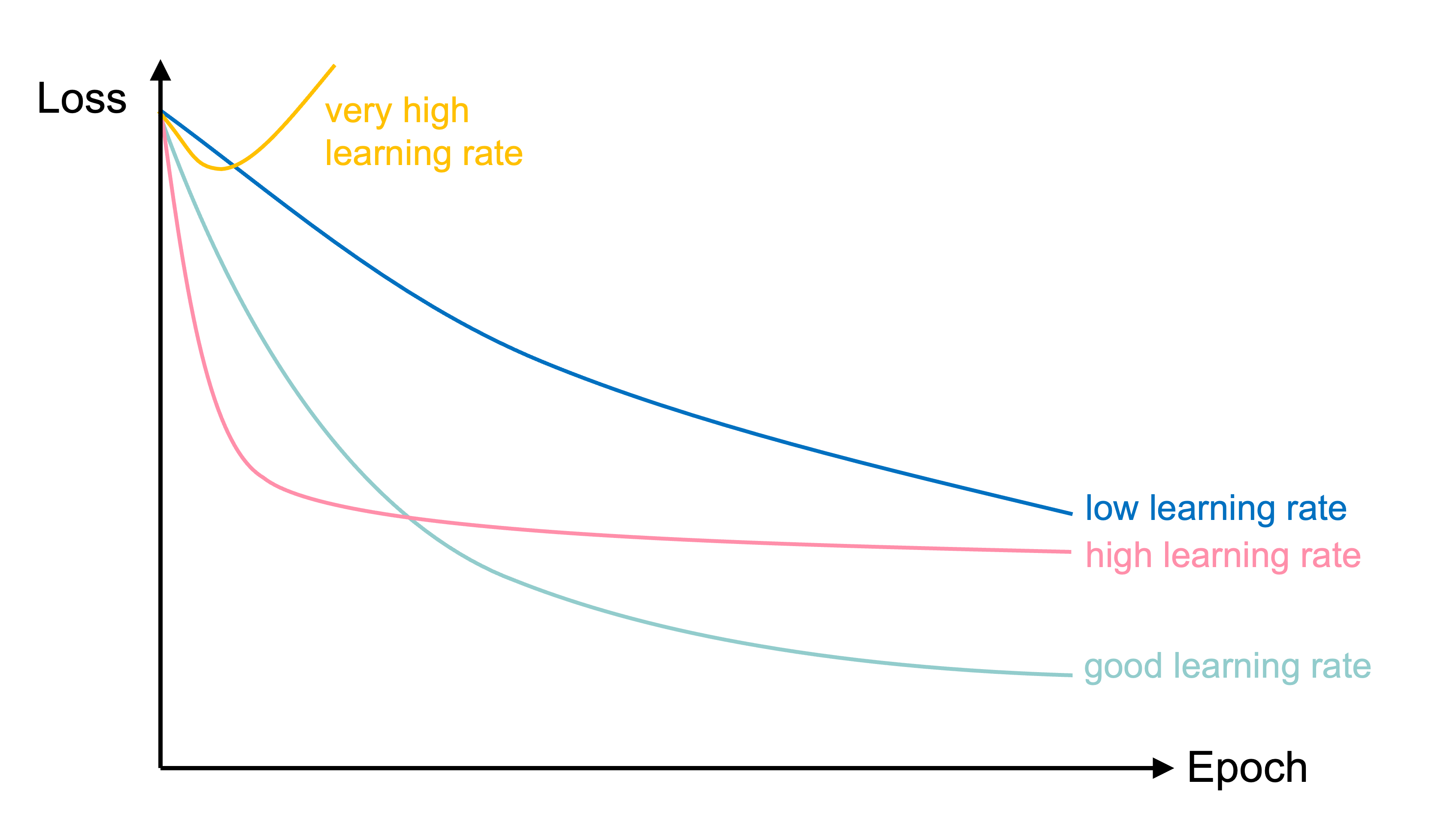
If the learning rate is too small, the subsequent NNs are too similar and it takes too long for the parameters to converge (and more likely to a local, not global, minimum). If the learning rate is too big, you could overshoot and the loss may increase.

Learning rates #2

Changing the learning rates for a robot arm.

“a nice way to see how the learning rate affects Stochastic Gradient Descent. we can use SGD to control a robot arm - minimizing the distance to the target as a function of the angles θᵢ. Too low a learning rate gives slow inefficient learning, too high and we see instability”

Learning rate schedule

Learning curves for various learning rates

In training the learning rate may be tweaked manually.

Loss and derivatives

How does gradient descent work mathematically?

Example: linear regression

\hat{y}(x) = w x + b

For some observation \{ x_i, y_i \}, the squared error loss is

\text{Loss}_i = (\hat{y}(x_i) - y_i)^2

For a batch of the first n observations the MSE loss is

\text{Loss}_{1:n} = \frac{1}{n} \sum_{i=1}^n (\hat{y}(x_i) - y_i)^2

Derivatives

Since \hat{y}(x) = w x + b,

\frac{\partial \hat{y}(x)}{\partial w} = x \text{ and } \frac{\partial \hat{y}(x)}{\partial b} = 1 .

As \text{Loss}_i = (\hat{y}(x_i) - y_i)^2, we know \frac{\partial \text{Loss}_i}{\partial \hat{y}(x_i) } = 2 (\hat{y}(x_i) - y_i) .

Chain rule

\frac{\partial \text{Loss}_i}{\partial \hat{y}(x_i) } = 2 (\hat{y}(x_i) - y_i), \,\, \frac{\partial \hat{y}(x)}{\partial w} = x , \, \text{ and } \, \frac{\partial \hat{y}(x)}{\partial b} = 1 .

Putting this together, we have

\frac{\partial \text{Loss}_i}{\partial w} = \frac{\partial \text{Loss}_i}{\partial \hat{y}(x_i) } \times \frac{\partial \hat{y}(x_i)}{\partial w} = 2 (\hat{y}(x_i) - y_i) \, x_i

and \frac{\partial \text{Loss}_i}{\partial b} = \frac{\partial \text{Loss}_i}{\partial \hat{y}(x_i) } \times \frac{\partial \hat{y}(x_i)}{\partial b} = 2 (\hat{y}(x_i) - y_i) .

We need non-zero derivatives

At all points in the neural network, we can’t have any derivative equal to 0. If it is 0 at any point, it becomes impossible for the model to learn.

This is why can’t use accuracy as the loss function for classification.

Also why we can have the dead ReLU problem.

Stochastic gradient descent (SGD)

Start with \boldsymbol{\theta}_0 = (w, b)^\top = (0, 0)^\top.

Randomly pick i=5, say x_i = 5 and y_i = 5.

\hat{y}(x_i) = 0 \times 5 + 0 = 0 \Rightarrow \text{Loss}_i = (0 - 5)^2 = 25.

The partial derivatives are \begin{aligned} \frac{\partial \text{Loss}_i}{\partial w} &= 2 (\hat{y}(x_i) - y_i) \, x_i = 2 \cdot (0 - 5) \cdot 5 = -50, \text{ and} \\ \frac{\partial \text{Loss}_i}{\partial b} &= 2 (0 - 5) = - 10. \end{aligned} The gradient is \nabla \text{Loss}_i = (-50, -10)^\top.

SGD, first iteration

Start with \boldsymbol{\theta}_0 = (w, b)^\top = (0, 0)^\top.

Randomly pick i=5, say x_i = 5 and y_i = 5.

The gradient is \nabla \text{Loss}_i = (-50, -10)^\top.

Use learning rate \eta = 0.01 to update \begin{aligned} \boldsymbol{\theta}_1 &= \boldsymbol{\theta}_0 - \eta \nabla \text{Loss}_i \\ &= \begin{pmatrix} 0 \\ 0 \end{pmatrix} - 0.01 \begin{pmatrix} -50 \\ -10 \end{pmatrix} \\ &= \begin{pmatrix} 0 \\ 0 \end{pmatrix} + \begin{pmatrix} 0.5 \\ 0.1 \end{pmatrix} = \begin{pmatrix} 0.5 \\ 0.1 \end{pmatrix}. \end{aligned}

SGD, second iteration

Start with \boldsymbol{\theta}_1 = (w, b)^\top = (0.5, 0.1)^\top.

Randomly pick i=9, say x_i = 9 and y_i = 17.

The gradient is \nabla \text{Loss}_i = (-223.2, -24.8)^\top.

Use learning rate \eta = 0.01 to update \begin{aligned} \boldsymbol{\theta}_2 &= \boldsymbol{\theta}_1 - \eta \nabla \text{Loss}_i \\ &= \begin{pmatrix} 0.5 \\ 0.1 \end{pmatrix} - 0.01 \begin{pmatrix} -223.2 \\ -24.8 \end{pmatrix} \\ &= \begin{pmatrix} 0.5 \\ 0.1 \end{pmatrix} + \begin{pmatrix} 2.232 \\ 0.248 \end{pmatrix} = \begin{pmatrix} 2.732 \\ 0.348 \end{pmatrix}. \end{aligned}

Batch gradient descent (BGD)

For the first n observations \text{Loss}_{1:n} = \frac{1}{n} \sum_{i=1}^n \text{Loss}_i so

\begin{aligned} \frac{\partial \text{Loss}_{1:n}}{\partial w} &= \frac{1}{n} \sum_{i=1}^n \frac{\partial \text{Loss}_{i}}{\partial w} = \frac{1}{n} \sum_{i=1}^n \frac{\partial \text{Loss}_{i}}{\hat{y}(x_i)} \frac{\partial \hat{y}(x_i)}{\partial w} \\ &= \frac{1}{n} \sum_{i=1}^n 2 (\hat{y}(x_i) - y_i) \, x_i . \end{aligned}

\begin{aligned} \frac{\partial \text{Loss}_{1:n}}{\partial b} &= \frac{1}{n} \sum_{i=1}^n \frac{\partial \text{Loss}_{i}}{\partial b} = \frac{1}{n} \sum_{i=1}^n \frac{\partial \text{Loss}_{i}}{\hat{y}(x_i)} \frac{\partial \hat{y}(x_i)}{\partial b} \\ &= \frac{1}{n} \sum_{i=1}^n 2 (\hat{y}(x_i) - y_i) . \end{aligned}

BGD, first iteration (\boldsymbol{\theta}_0 = \boldsymbol{0})

	x	y	loss	dL/dw	dL/db
0	1	0.99	0.98	-1.98	-1.98
1	2	3.00	9.02	-12.02	-6.01
2	3	5.01	25.15	-30.09	-10.03

So \nabla \text{Loss}_{1:3} is

nabla = np.array([df["dL/dw"].mean(), df["dL/db"].mean()])
nabla

array([-14.69,  -6.  ])

so with \eta = 0.1 then \boldsymbol{\theta}_1 becomes

theta_1 = theta_0 - 0.1 * nabla
theta_1

array([1.47, 0.6 ])

BGD, second iteration

	x	y	y_hat	loss	dL/dw	dL/db
0	1	0.99	2.07	1.17	2.16	2.16
1	2	3.00	3.54	0.29	2.14	1.07
2	3	5.01	5.01	0.00	-0.04	-0.01

So \nabla \text{Loss}_{1:3} is

nabla = np.array([df["dL/dw"].mean(), df["dL/db"].mean()])
nabla

array([1.42, 1.07])

so with \eta = 0.1 then \boldsymbol{\theta}_2 becomes

theta_2 = theta_1 - 0.1 * nabla
theta_2

array([1.33, 0.49])

Glossary

batch gradient descent
batches, batch size
global minimum, local minimum
gradient-based learning, hill-climbing
learning rate, learning rate schedule
plateau
stochastic gradient descent
mini-batch gradient descent