Generative Networks
ACTL3143 & ACTL5111 Deep Learning for Actuaries
Generative Adversarial Networks
GANs consist of two neural networks, a generator, and a discriminator, and they are trained simultaneously through adversarial training. The generator takes in random noise and generates a synthetic data observation. The goal of the generator is to learn how to generate synthetic data that resembles actual data very well. The discriminator distinguishes between real and synthetic data and classifies them as ‘real’ or ‘fake’. The goal of the discriminator is to correctly identify whether the input is real or synthetic. An equilibrium is reached when the generator is able to generate data that very well resembles actual data and the discriminator is unable to distinguish them with high confidence.
GAN faces
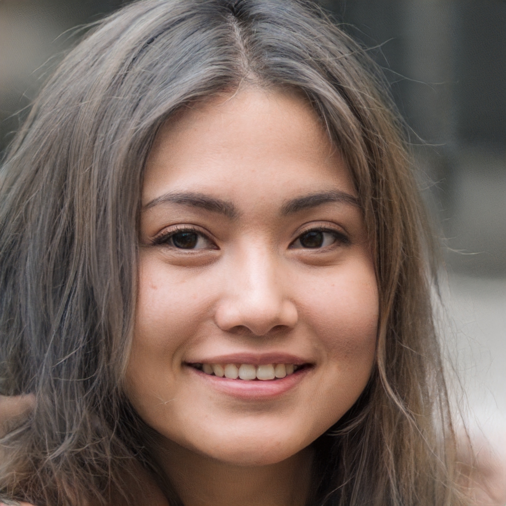

Try out https://www.whichfaceisreal.com.
Example StyleGAN2-ADA outputs
GAN structure
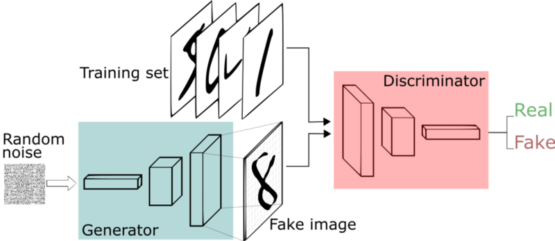
Two NNs in the structure:
- Generator: creates fake data (fake images)
- input: random noise
- output: fake data (fake image)
- Discriminator: tries to determine whether the input is real or fake
- input: data (image)
- output: binary classification
GAN intuition
We want to train both the generator and the discriminator:
- Train the generator to generate more realistic images
- Train the discriminator to get better at distinguishing between real and fake images
Intuition about GANs
- A forger creates a fake Picasso painting to sell to an art dealer.
- The art dealer assesses the painting.
How they best each other:
- The art dealer is given both authentic paintings and fake paintings to look at. Later on, the validity of his assessment is evaluated and he trains to become better at detecting fakes. Over time, he becomes increasingly expert at authenticating Picasso’s artwork.
- The forger receives an assessment from the art dealer every time he gives him a fake. He knows he has to perfect his craft if the art dealer can detect his fake. He becomes increasingly adept at imitating Picasso’s style.
Generative adversarial networks
- A GAN is made up of two parts:
- Generator network: the forger. Takes a random point in the latent space, and decodes it into a synthetic data/image.
- Discriminator network (or adversary): the expert. Takes a data/image and decides whether it exists in the original data set (the training set) or was created by the generator network.
Discriminator
lrelu = layers.LeakyReLU(alpha=0.2)

discriminator = keras.Sequential([
    keras.Input(shape=(28, 28, 1)),
    layers.Conv2D(64, 3, strides=2, padding="same", activation=lrelu),
    layers.Conv2D(128, 3, strides=2, padding="same", activation=lrelu),
    layers.GlobalMaxPooling2D(),
    layers.Dense(1)])

discriminator.summary()
Generator
latent_dim = 128
generator = keras.Sequential([
    layers.Dense(7 * 7 * 128, input_dim=latent_dim, activation=lrelu),
    layers.Reshape((7, 7, 128)),
    layers.Conv2DTranspose(128, 4, strides=2, padding="same", activation=lrelu),
    layers.Conv2DTranspose(128, 4, strides=2, padding="same", activation=lrelu),
    layers.Conv2D(1, 7, padding="same", activation="sigmoid")])
generator.summary()
Training GANs
GAN cost functions
GAN - Schematic process
First step: Training discriminator:
- Draw random points in the latent space (random noise).
- Use generator to generate data from this random noise.
- Mix generated data with real data and input them into the discriminator. The training targets are the correct labels of real data or fake data. Use discriminator to give feedback on the mixed data whether they are real or synthetic. Train discriminator to minimize the loss function which is the difference between the discriminator’s feedback and the correct labels.
GAN - Schematic process II
Second step: Training generator:
- Draw random points in the latent space and generate data with generator.
- Use discriminator to give feedback on the generated data. What the generator tries to achieve is to fool the discriminator into thinking all generated data are real data. Train generator to minimize the loss function which is the difference between the discriminator’s feedback and the desired feedback: “All data are real data” (which is not true).
GAN - Schematic process III
- When training, the discriminator may end up dominating the generator because the loss function for training the discriminator tends to zero faster. In that case, try reducing the learning rate and increasing the dropout rate of the discriminator.
- There are a few tricks for implementing GANs such as introducing stochasticity by adding random noise to the labels for the discriminator, using stride instead of pooling in the discriminator, using kernel size that is divisible by stride size, etc.
Train step
# Separate optimisers for discriminator and generator.
d_optimizer = keras.optimizers.Adam(learning_rate=0.0003)
g_optimizer = keras.optimizers.Adam(learning_rate=0.0004)

# Instantiate a loss function.
loss_fn = keras.losses.BinaryCrossentropy(from_logits=True)

@tf.function
def train_step(real_images):
  # Sample random points in the latent space
  random_latent_vectors = tf.random.normal(shape=(batch_size, latent_dim))
  # Decode them to fake images
  generated_images = generator(random_latent_vectors)
  # Combine them with real images
  combined_images = tf.concat([generated_images, real_images], axis=0)

  # Assemble labels discriminating real from fake images
  labels = tf.concat([
    tf.zeros((batch_size, 1)),
    tf.ones((real_images.shape[0], 1))], axis=0)

  # Add random noise to the labels - important trick!
  labels += 0.05 * tf.random.uniform(labels.shape)

  # Train the discriminator
  with tf.GradientTape() as tape:
    predictions = discriminator(combined_images)
    d_loss = loss_fn(labels, predictions)
  grads = tape.gradient(d_loss, discriminator.trainable_weights)
  d_optimizer.apply_gradients(zip(grads, discriminator.trainable_weights))

  # Sample random points in the latent space
  random_latent_vectors = tf.random.normal(shape=(batch_size, latent_dim))

  # Assemble labels that say "all real images"
  misleading_labels = tf.ones((batch_size, 1))

  # Train the generator (note that we should *not* update the weights
  # of the discriminator)!
  with tf.GradientTape() as tape:
    predictions = discriminator(generator(random_latent_vectors))
    g_loss = loss_fn(misleading_labels, predictions)

  grads = tape.gradient(g_loss, generator.trainable_weights)
  g_optimizer.apply_gradients(zip(grads, generator.trainable_weights))
  return d_loss, g_loss, generated_images
Grab the data
# Prepare the dataset.
# We use both the training & test MNIST digits.
batch_size = 64
(x_train, _), (x_test, _) = keras.datasets.mnist.load_data()
all_digits = np.concatenate([x_train, x_test])
all_digits = all_digits.astype("float32") / 255.0
all_digits = np.reshape(all_digits, (-1, 28, 28, 1))
dataset = tf.data.Dataset.from_tensor_slices(all_digits)
dataset = dataset.shuffle(buffer_size=1024).batch(batch_size)

# In practice you need at least 20 epochs to generate nice digits.
epochs = 1
save_dir = "./"
Train the GAN
%%time
for epoch in range(epochs):
  for step, real_images in enumerate(dataset):
    # Train the discriminator & generator on one batch of real images.
    d_loss, g_loss, generated_images = train_step(real_images)

    # Logging.
    if step % 200 == 0:
      # Print metrics
      print(f"Discriminator loss at step {step}: {d_loss:.2f}")
      print(f"Adversarial loss at step {step}: {g_loss:.2f}")
      break # Remove this if really training the GAN
Conditional GANs
Unconditional vs conditional generation
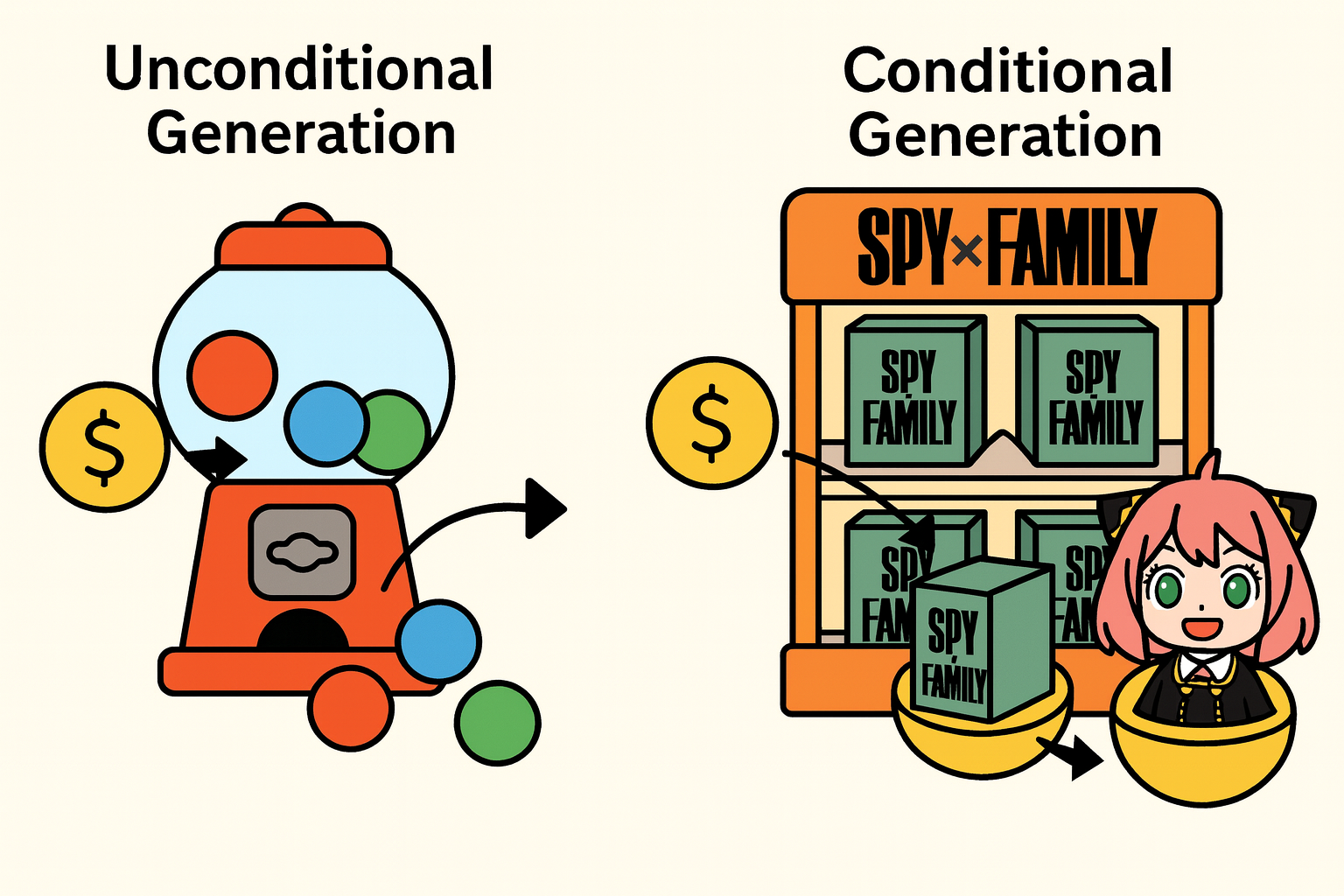
- Unconditional generation
- Complete randomness
- Conditional generation
- Randomness that is bounded in some way. You don’t know what you’re getting, but you know it is in a certain category.
Hurricane example data
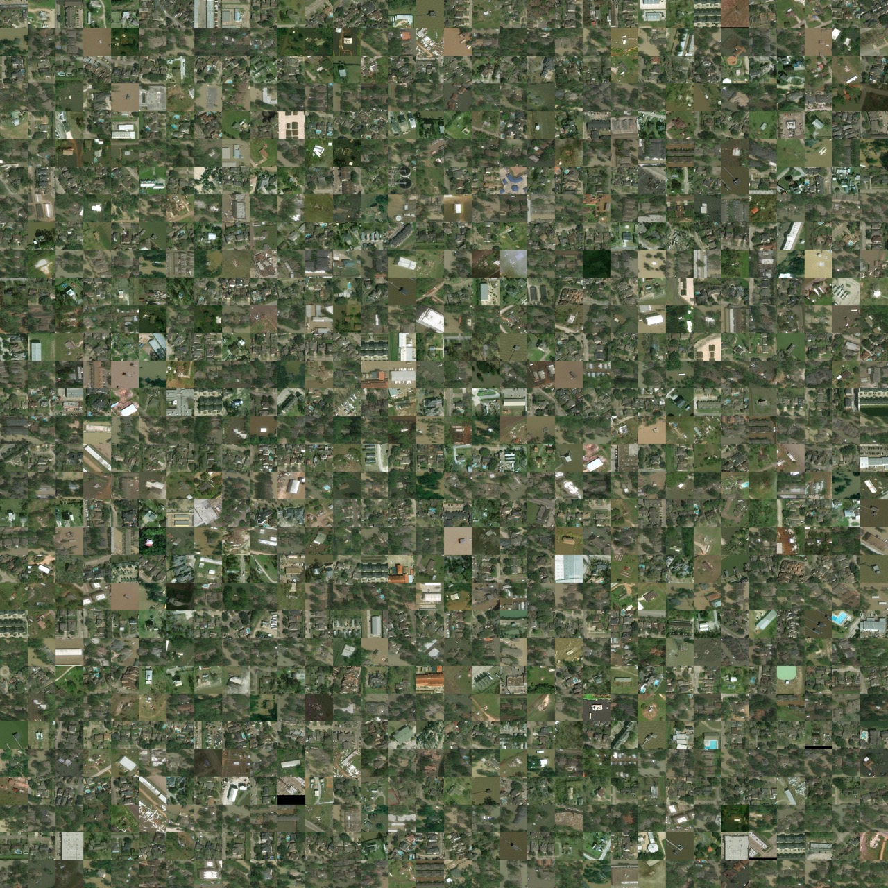
This is a labelled dataset of satellite images; some are under normal circumstances, and some are after a hurricane occurred.
Hurricane example
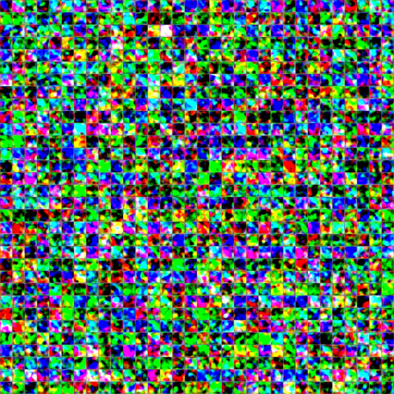
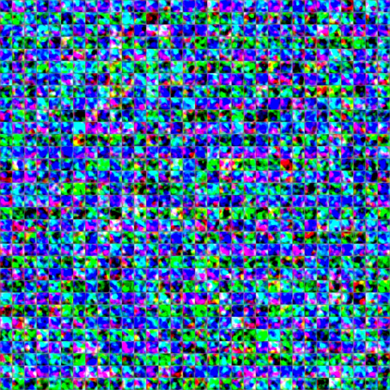
The original dataset was input to a conditional GAN. The GAN starts off by generating random images.
Hurricane example (after 54s)
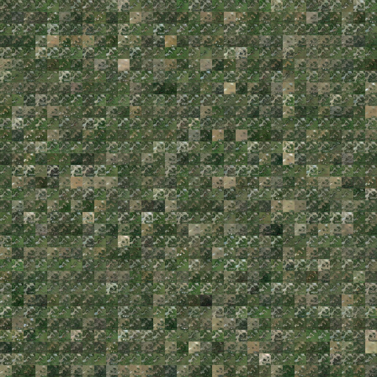
After 1 iteration, the fake images start to look more like the original dataset, but still far off.
Hurricane example (after 21m)
Hurricane example (after 47m)
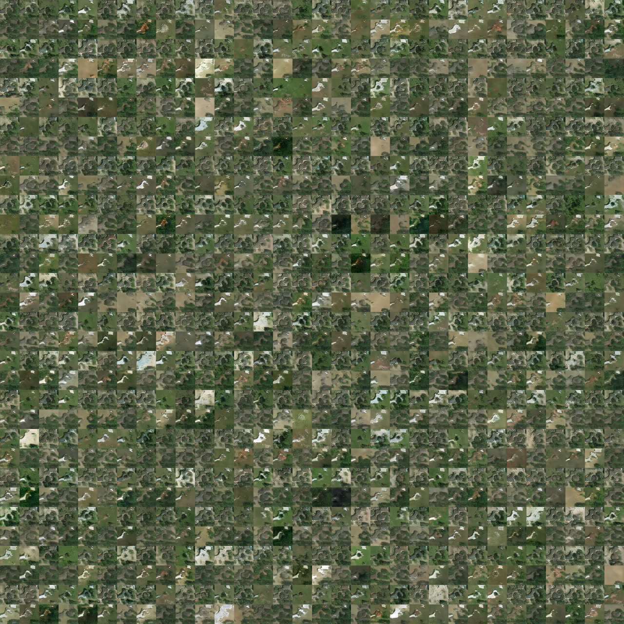
Hurricane example (after 4h10m)
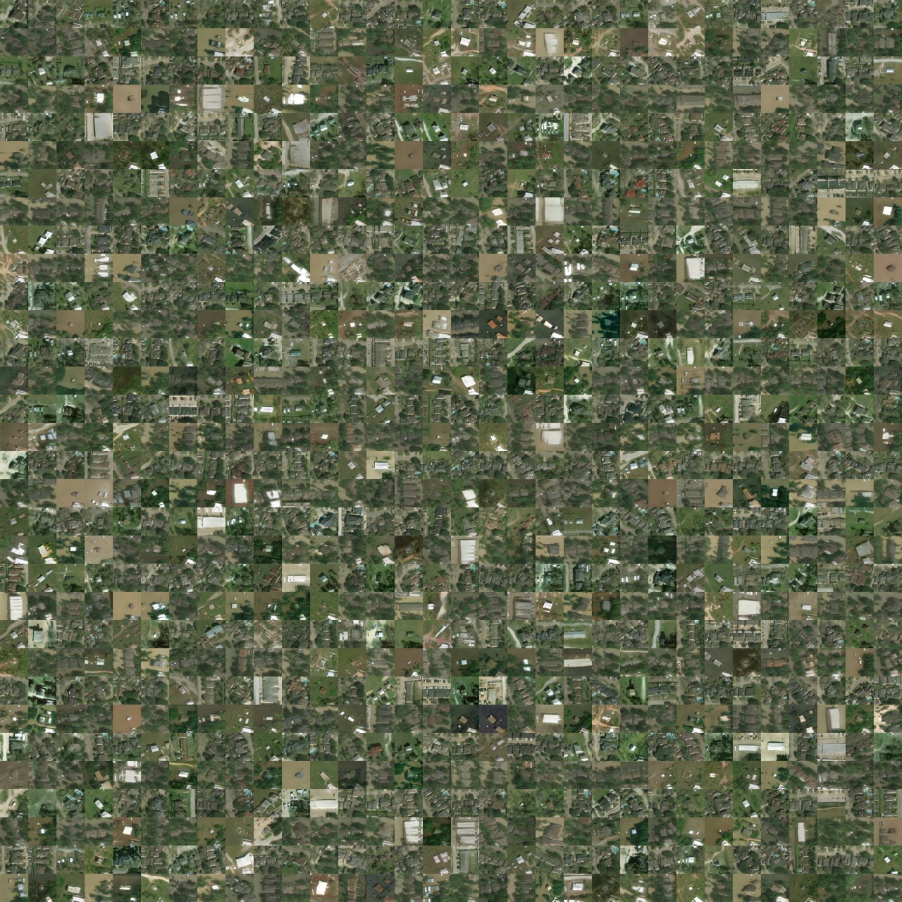
Hurricane example (after 14h41m)
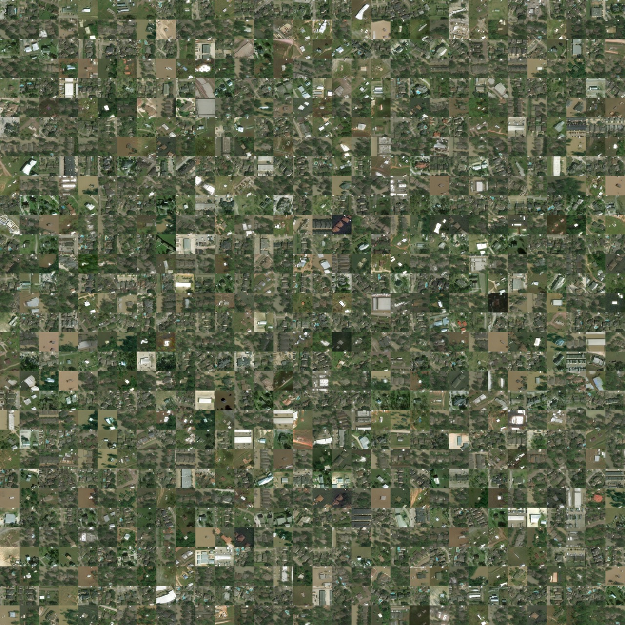
By the end (over 14 hours!), the fake images look much more realistic — if you zoom in, you can see that they are certainly not perfect, but have much more detail and variety than the previous iterations shown.
The benefit of training a conditional GAN is that we can ask it to generate new images that would come from each category: occurred after a hurricane or not.
Image-to-image translation
Example: Deoldify images #1
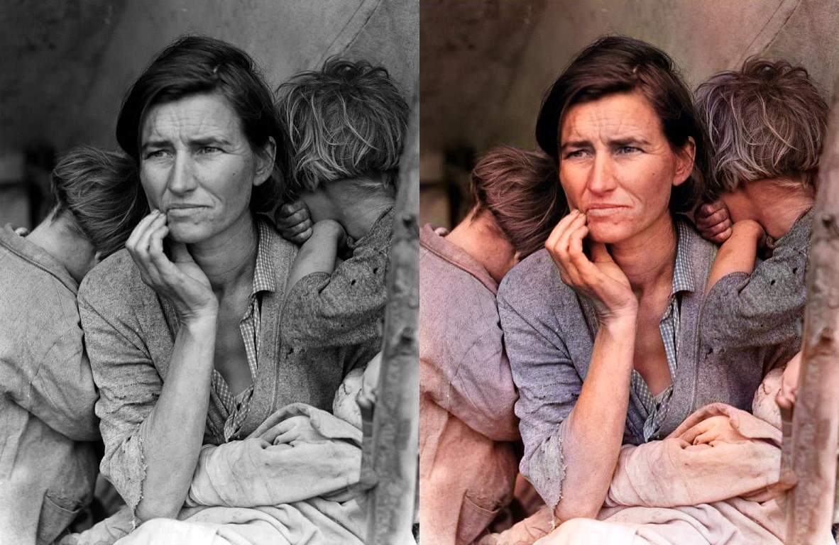
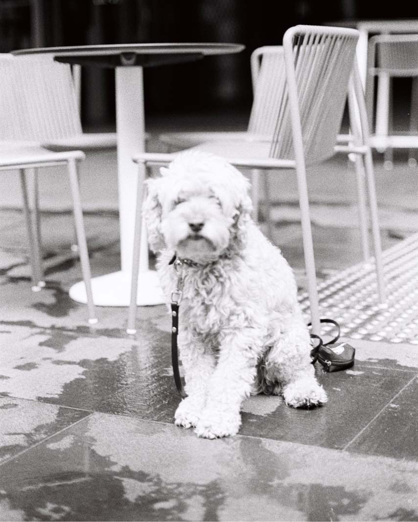
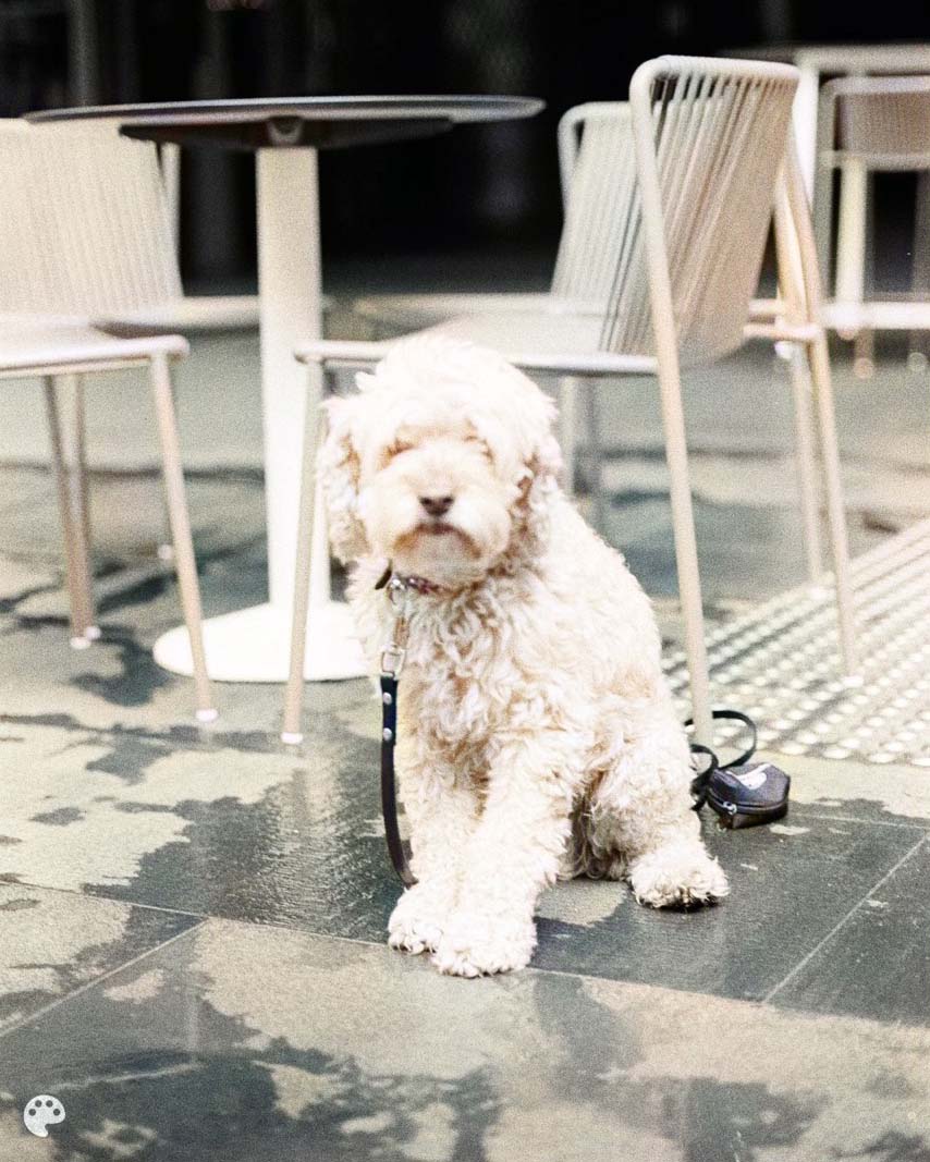
Here, the conditional GAN is trained on the specific image we see on the left. The “category” is the black and white image itself, and it is trained to colourise the image.
Example: Deoldify images #2

Example: Deoldify images #3
Explore the latent space
Can I get a GAN to produce a fake face that looks like mine?
The initial image is a randomly generated face.
Generator can’t generate everything


Problems with GANs
They are slow to train
StyleGAN2-ADA training times on V100s (1024x1024):
| GPUs | 1000 kimg | 25000 kimg | sec / kimg | GPU mem | CPU mem |
|---|---|---|---|---|---|
| 1 | 1d 20h | 46d 03h | 158 | 8.1 GB | 5.3 GB |
| 2 | 23h 09m | 24d 02h | 83 | 8.6 GB | 11.9 GB |
| 4 | 11h 36m | 12d 02h | 40 | 8.4 GB | 21.9 GB |
| 8 | 5h 54m | 6d 03h | 20 | 8.3 GB | 44.7 GB |
Uncertain convergence
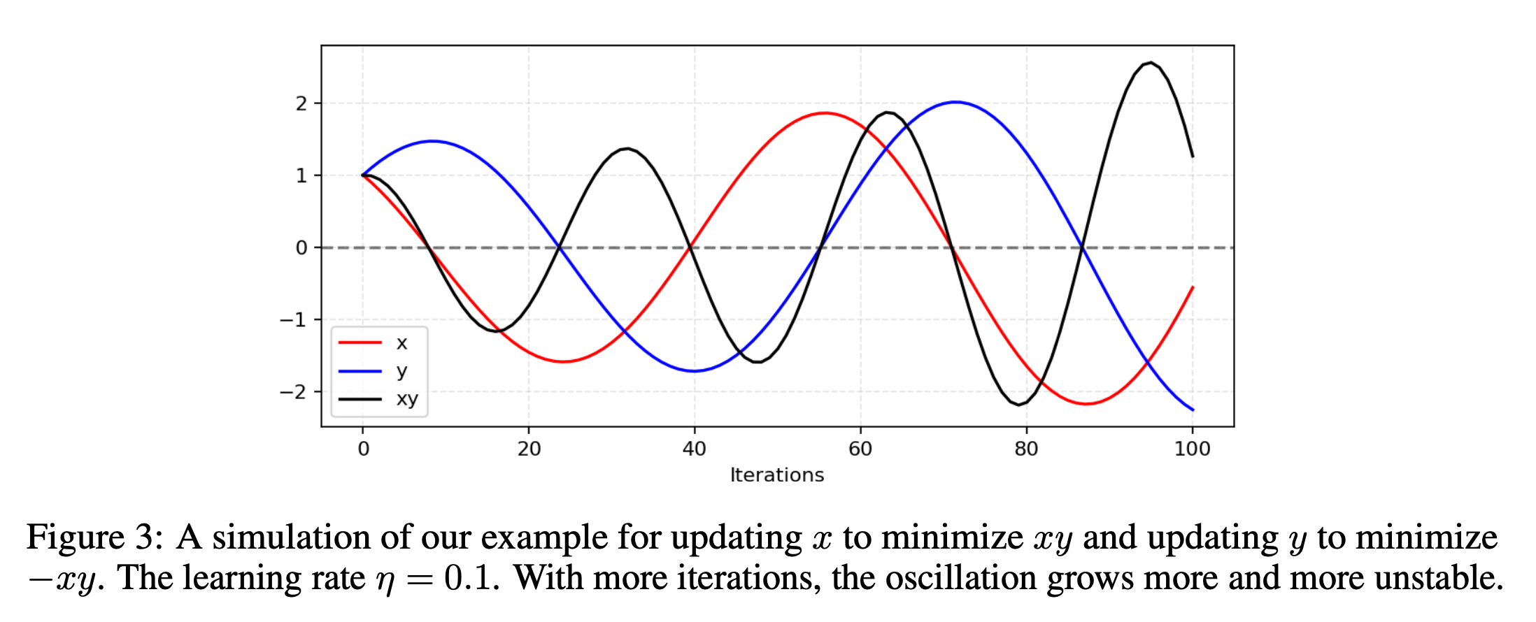
Converges to a Nash equilibrium, if at all.
Mode collapse
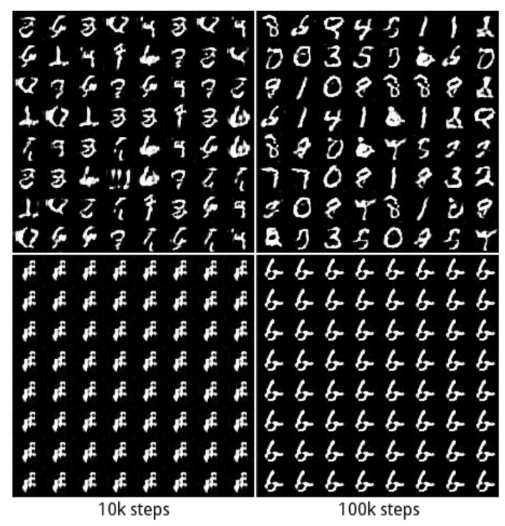
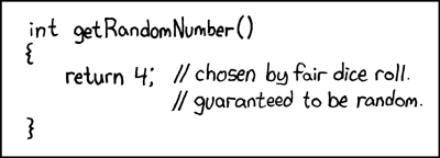
You want the GAN to create lots of different realistic-looking faces. The example above shows how the GAN was unable to create a variety of images, and just created the same one over and over.
Generation is harder

# Separate optimisers for discriminator and generator.
d_optimizer = keras.optimizers.Adam(learning_rate=0.0003)
g_optimizer = keras.optimizers.Adam(learning_rate=0.0004)
The two NNs have to learn at the right rates. One can’t dominate the other; otherwise the whole process falls apart. Finding those learning rates is difficult.
Advanced image layers
Conv2D
GlobalMaxPool2D
Conv2DTranspose
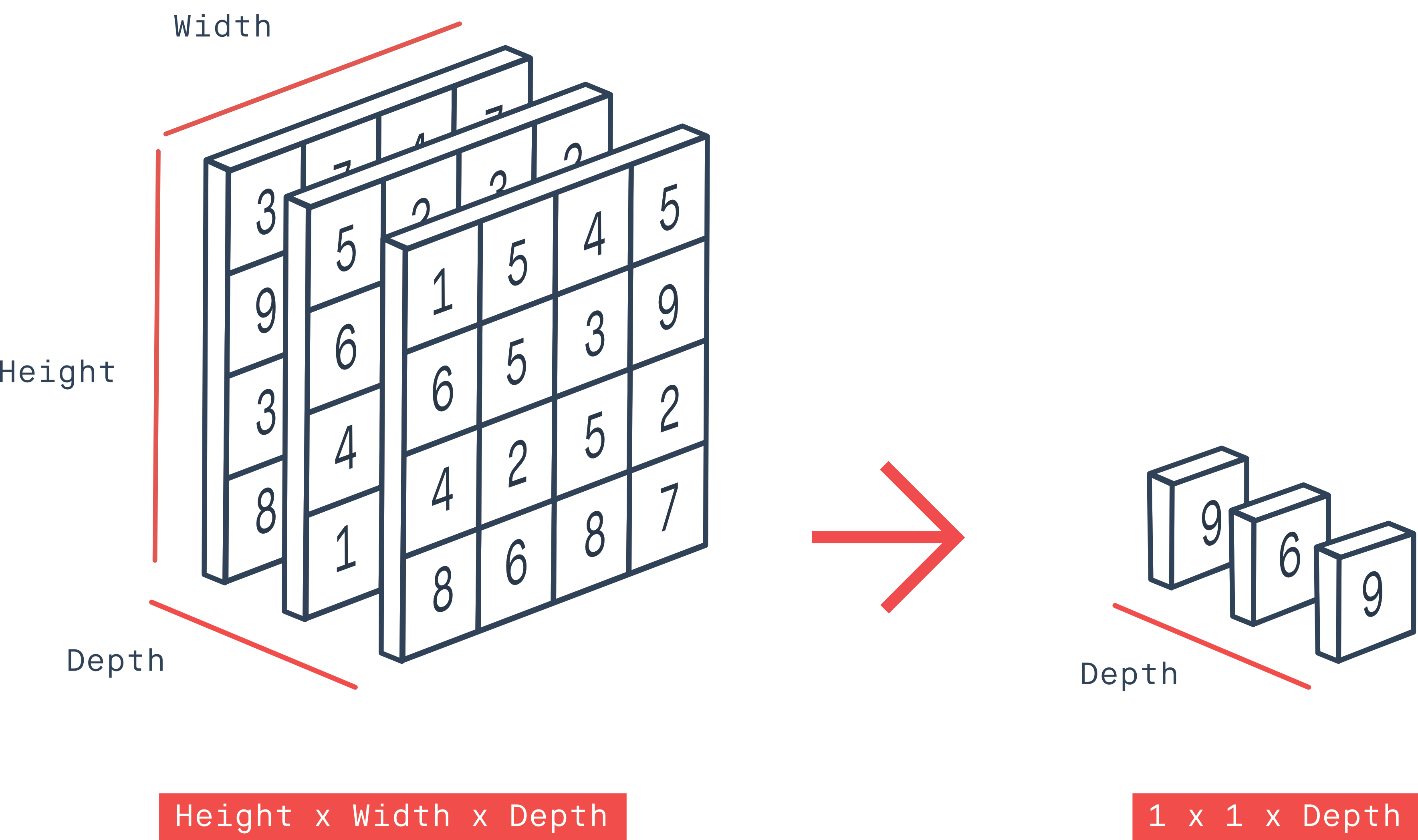
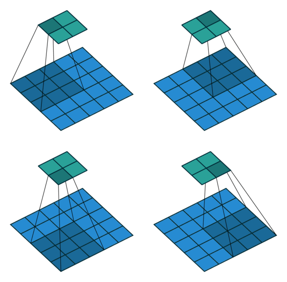
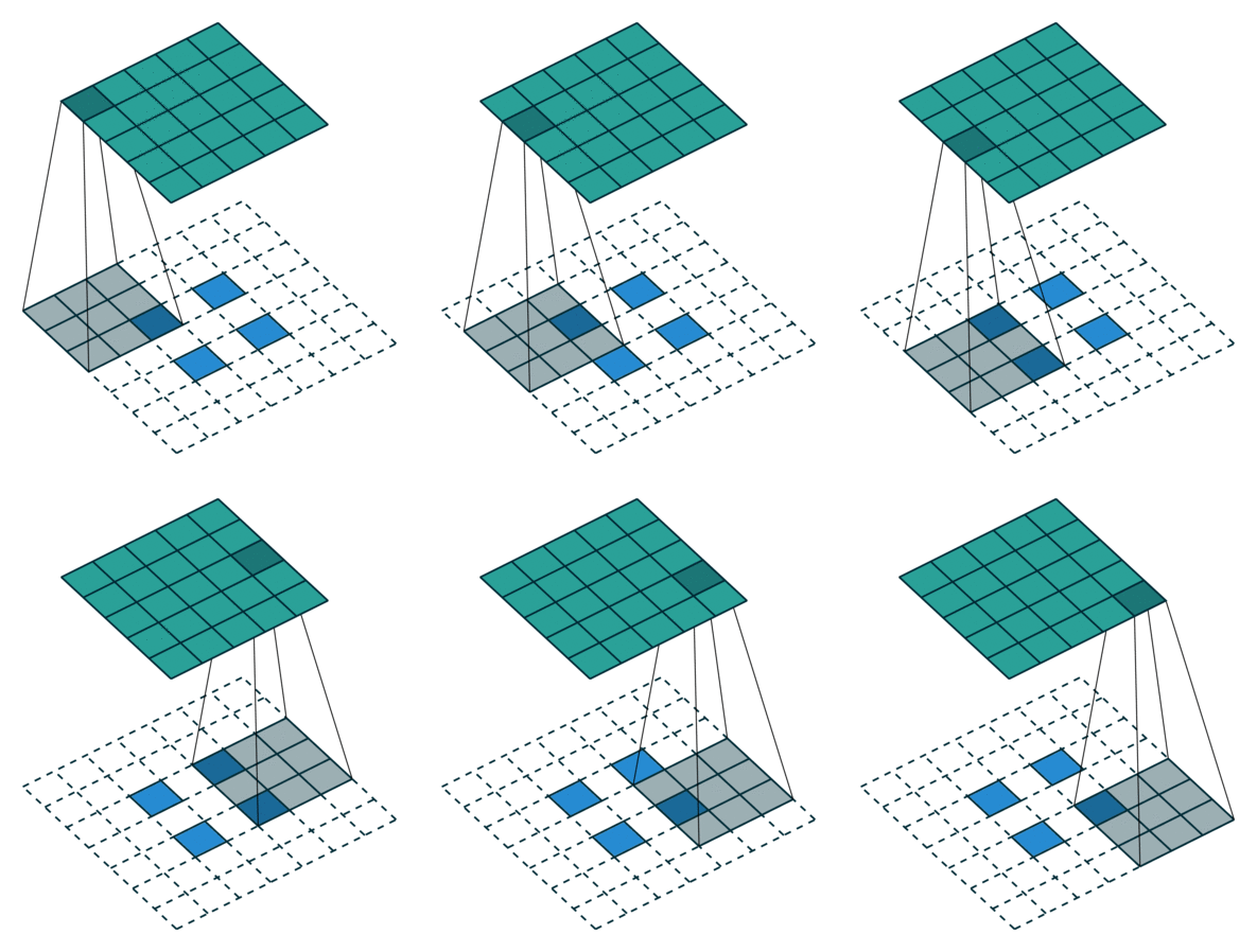
In the course so far, we have been looking at reducing images to numbers (Figures 1 and 2). With GANs, the opposite needs to be done (Figure 3). This is a much more complex process.
Vanishing gradients I
BCE Loss and vanishing gradients 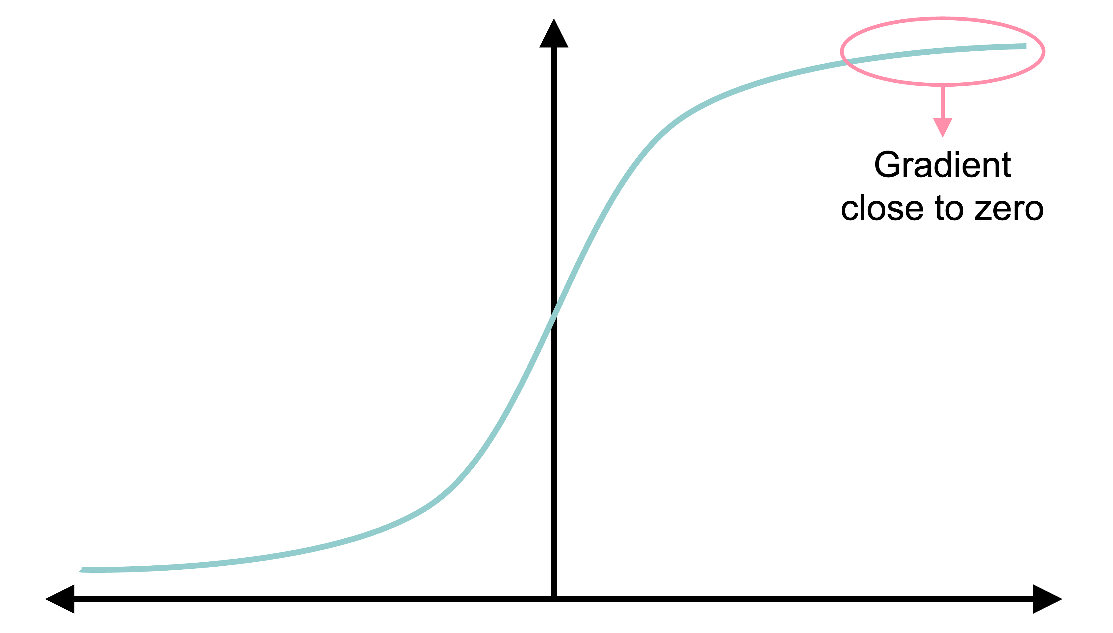
Vanishing gradients II
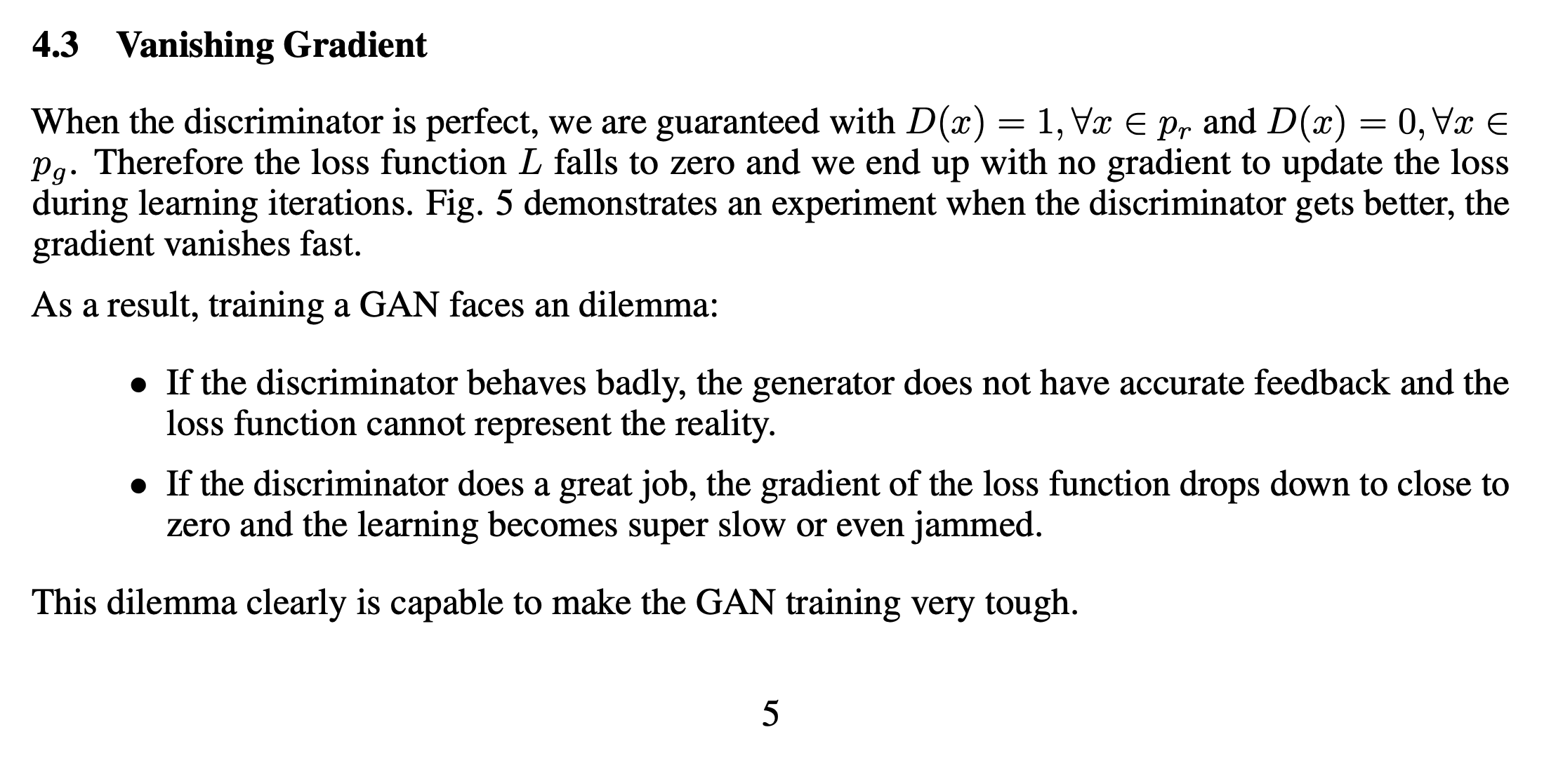
Wasserstein GAN
We’re comparing distributions
Trying to minimise the distance between the distribution of generated samples and the distribution of real data.
Vanilla GAN is equivalent to minimising the Jensen–Shannon Divergence between the two.
An alternative distance between distributions is the Wasserstein distance.
Discriminator Critic
Critic D : \text{Input} \to \mathbb{R} how “authentic” the input looks. It can’t discriminate real from fake exactly.
Critic’s goal is
\max_{D \in \mathscr{D}} \mathbb{E}[ D(X) ] - \mathbb{E}[ D(G(Z)) ]
where \mathscr{D} is space of 1-Lipschitz functions. Either use gradient clipping or penalise gradients far from 1:
\max_{D} \mathbb{E}[ D(X) ] - \mathbb{E}[ D(G(Z)) ] + \lambda \mathbb{E} \Bigl[ ( \bigl|\bigl| \nabla D \bigr|\bigr| - 1)^2 \Bigr] .
GANs with differential privacy
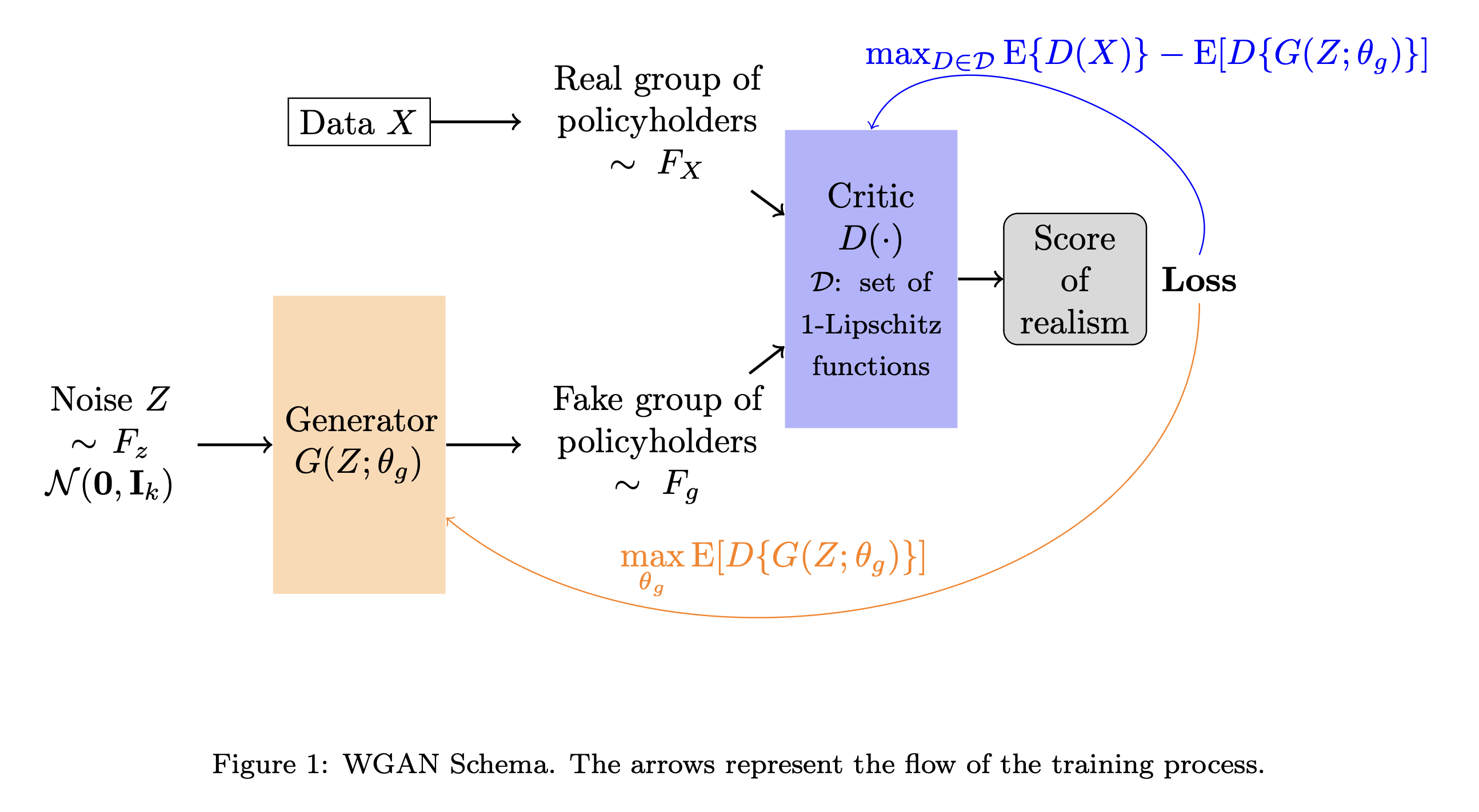
In some cases, we can’t use real policyholder data; it’s a breach of privacy. The goal is to make a GAN that learns the characteristics of the policy data, generate a fake dataset of poliycholders that resembles the real one; then the fake data can be given to anyone.
- Differential privacy
- You don’t want any of the real policyholders to leak into the fake dataset. How do we leverage the data without leaking it?
Links
- Dongyu Liu (2021), TadGAN: Time Series Anomaly Detection Using Generative Adversarial Networks
- Jeff Heaton (2022), GANs for Tabular Synthetic Data Generation (7.5)
- Jeff Heaton (2022), GANs to Enhance Old Photographs Deoldify (7.4)
Language Models
Generative deep learning
- Using AI as augmented intelligence rather than artificial intelligence.
- Use of deep learning to augment creative activities such as writing, music and art, to generate new things.
- Some applications: text generation, deep dreaming, neural style transfer, variational autoencoders and generative adversarial networks.
Text generation
Generating sequential data is the closest computers get to dreaming.
- Generate sequence data: Train a model to predict the next token or next few tokens in a sentence, using previous tokens as input.
- A network that models the probability of the next tokens given the previous ones is called a language model.
GPT-3 is a 175 billion parameter text-generation model trained by the startup OpenAI on a large text corpus of digitally available books, Wikipedia and web crawling. GPT-3 made headlines in 2020 due to its capability to generate plausible-sounding text paragraphs on virtually any topic.
Word-level language model
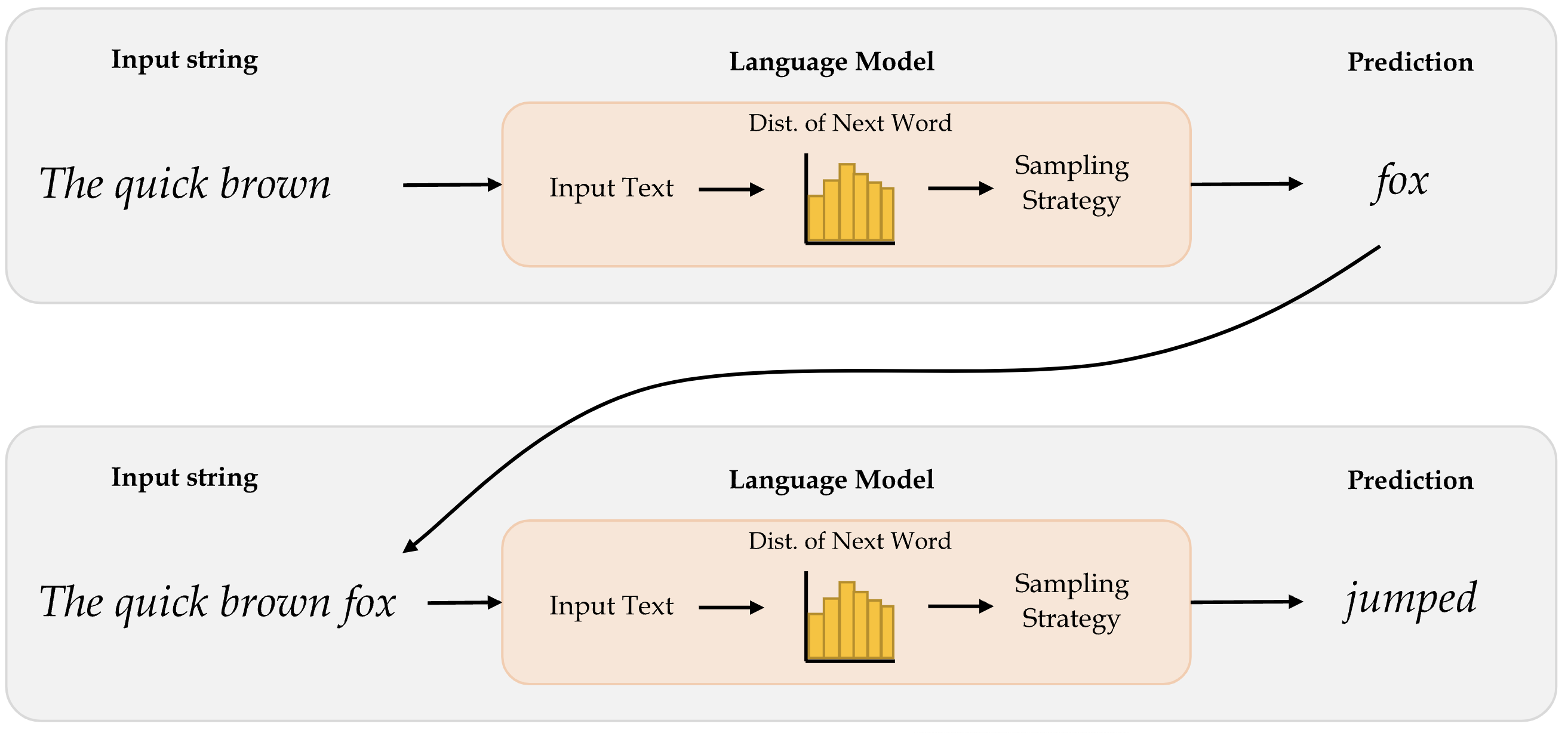
How word-level language models work:
- Takes in the input text and generates the probability distribution of the next word. This distribution tells us how likely a certain word is to be the next word.
- Implements an appropriate sampling strategy to select the next word.
- Once the next word is predicted, it is appended to the input text and then passed in to the model again to predict the next word.
The idea is to predict the words sequentially.
Character-level language model
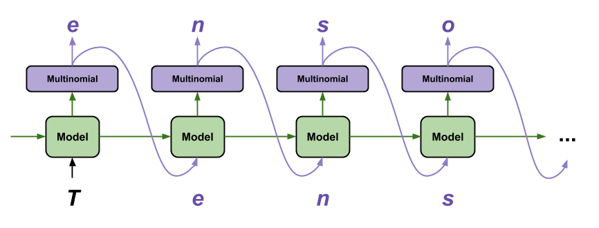
Character-level language predicts the next character given a certain input character. They capture patterns at a more granular level and do not aim to capture semantics of words.
Useful for speech recognition
| RNN output | Decoded Transcription |
|---|---|
| what is the weather like in bostin right now | what is the weather like in boston right now |
| prime miniter nerenr modi | prime minister narendra modi |
| arther n tickets for the game | are there any tickets for the game |
The above example shows how RNN predictions (for sequential data processing) can be improved by fixing errors using a language model.
Generating Shakespeare I
The following is an example of how a language model that is trained on works of Shakespeare starts predicting words after we input a string. This is an example of a character-level prediction, where we aim to predict the most likely character, not the word.
ROMEO:
Why, sir, what think you, sir?
AUTOLYCUS:
A dozen; shall I be deceased.
The enemy is parting with your general,
As bias should still combit them offend
That Montague is as devotions that did satisfied;
But not they are put your pleasure.
Generating Shakespeare II
DUKE OF YORK:
Peace, sing! do you must be all the law;
And overmuting Mercutio slain;
And stand betide that blows which wretched shame;
Which, I, that have been complaints me older hours.
LUCENTIO:
What, marry, may shame, the forish priest-lay estimest you, sir,
Whom I will purchase with green limits o’ the commons’ ears!
Generating Shakespeare III
ANTIGONUS:
To be by oath enjoin’d to this. Farewell!
The day frowns more and more: thou’rt like to have
A lullaby too rough: I never saw
The heavens so dim by day. A savage clamour!
[Exit, pursued by a bear]
Sampling strategy
The sampling strategy refers to how we pick the next word/character as the prediction after observing the distribution. There are different sampling strategies and they aim to serve different levels of trade-offs between exploration and exploitation when generating text sequences.
Sampling strategy
- Greedy sampling will choose the token with the highest probability. It makes the resulting sentence repetitive and predictable.
- Stochastic sampling: if a word has probability 0.3 of being next in the sentence according to the model, we’ll choose it 30% of the time. But the result is still not interesting enough and still quite predictable.
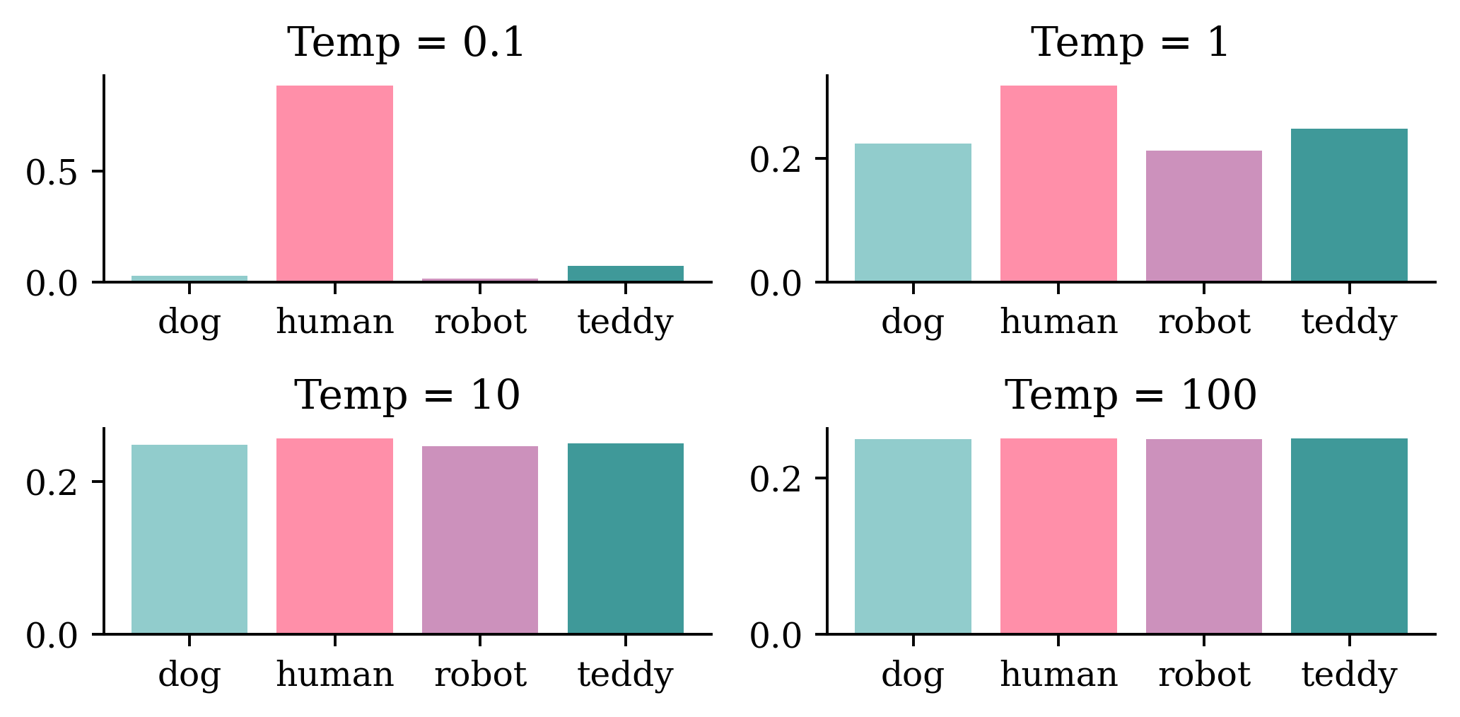
- Use a softmax temperature to control the randomness. More randomness results in more surprising and creative sentences.
Softmax temperature
- The softmax temperature is a parameter that controls the randomness of the next token.
- The formula is: \text{softmax}_\text{temperature}(x) = \frac{\exp(x / \text{temperature})}{\sum_i \exp(x_i / \text{temperature})}
“I am a” …
The graphical illustration above shows how the distribution of words change with different levels of temperature values. Higher levels of temperatures result in less predictable(more interesting) outcomes. If we continue to increase the temperature, after a certain point, outcomes will be picked completely at random. The predictions after this point might not be meaningful. Hence, attention to the trade-off between predictability and creativity is important when deciding the temperature.
Setting \text{Temp} = 1 returns the normal softmax function.
Generating Laub (temp = 0.01)
Here I have trained a neural network based on the transcripts of my lecture recordings. Given the starting point “In today’s lecture we will”, I asked it to generate very different completions at varying temperatures. Setting temperature to 0.25 may give interesting outputs compared to 0.01, and 0.50 may give more creative outputs compared to 0.25. However, when we keep on increasing temperature, the neural network starts giving out meaningless sequences.
In today’s lecture we will be different situation. So, next one is what they rective that each commit to be able to learn some relationships from the course, and that is part of the image that it’s very clese and black problems that you’re trying to fit the neural network to do there instead of like a specific though shef series of layers mean about full of the chosen the baseline of car was in the right, but that’s an important facts and it’s a very small summary with very scrort by the beginning of the sentence.
Generating Laub (temp = 0.25)
In today’s lecture we will decreas before model that we that we have to think about it, this mightsks better, for chattely the same project, because you might use the test set because it’s to be picked up the things that I wanted to heard of things that I like that even real you and you’re using the same thing again now because we need to understand what it’s doing the same thing but instead of putting it in particular week, and we can say that’s a thing I mainly link it’s three columns.
Generating Laub (temp = 0.5)
In today’s lecture we will probably the adw n wait lots of ngobs teulagedation to calculate the gradient and then I’ll be less than one layer the next slide will br input over and over the threshow you ampaigey the one that we want to apply them quickly. So, here this is the screen here the main top kecw onct three thing to told them, and the output is a vertical variables and Marceparase of things that you’re moving the blurring and that just data set is to maybe kind of categorical variants here but there’s more efficiently not basically replace that with respect to the best and be the same thing.
Generating Laub (temp = 1)
In today’s lecture we will put it different shates to touch on last week, so I want to ask what are you object frod current. They don’t have any zero into it, things like that which mistakes. 10 claims that the average version was relden distever ditgs and Python for the whole term wo long right to really. The name of these two options. There are in that seems to be modified version. If you look at when you’re putting numbers into your, that that’s over. And I went backwards, up, if they’rina functional pricing working with.
Generating Laub (temp = 1.5)
In today’s lecture we will put it could be bedinnth. Lowerstoriage nruron. So rochain the everything that I just sGiming. If there was a large. It’s gonua draltionation. Tow many, up, would that black and 53% that’s girter thankAty will get you jast typically stickK thing. But maybe. Anyway, I’m going to work on this libry two, past, at shit citcs jast pleming to memorize overcamples like pre pysing, why wareed to smart a one in this reportbryeccuriay.
Copilot’s “Conversation Style”
In Copilot, we can choose a “conversation style”: more creative, more balanced, and more precise. The different options might just reflect different temperatures.

Generate the most likely sequence
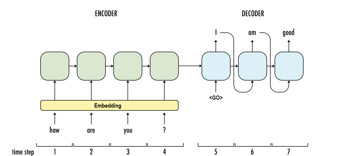
Similar to other sequence generating tasks such as generating the next word or generating the next character, generating an entire sequence of words is also useful. The task involves generating the most likely sequence after observing model predictions.
Beam search
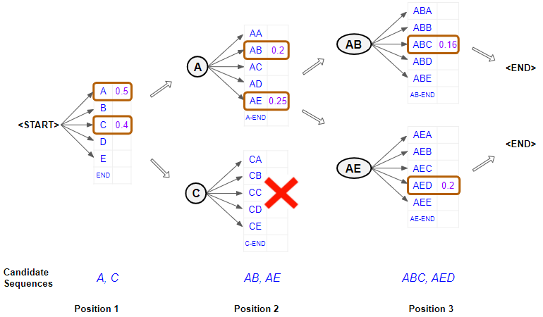
Instead of trying to carry forward only the highest probable prediction, beam search carries forward several high probable predictions, and then decide the highest probable combination of predictions. Beam search helps expand the exploration horizon for predictions which can contribute to more contextually relevant model predictions. However, this comes at a certain computational complexity.
Transformers
Transformers are a special type of neural networks that are proven to be highly effective in NLP tasks. They can capture long-run dependencies in the sequential data that is useful for generating predictions with contextual meaning. It makes use of the self-attention mechanism which studies all inputs in the sequence together, tries to understand the dependencies among them, and then utilizes the information about long-run dependencies to predict the output sequence.
Transformer architecture
GPT makes use of a mechanism known as attention, which removes the need for recurrent layers (e.g., LSTMs). It works like an information retrieval system, utilizing queries, keys, and values to decide how much information it wants to extract from each input token.
Attention heads can be grouped together to form what is known as a multihead attention layer. These are then wrapped up inside a Transformer block, which includes layer normalization and skip connections around the attention layer. Transformer blocks can be stacked to create very deep neural networks.
Highly recommended viewing: Iulia Turk (2021), Transfer learning and Transformer models, ML Tech Talks.
🤗 Transformers package
The following code uses the transformers library from Hugging Face to create a text generation pipeline using the GPT-2 (Generative Pre-trained Transformer 2).
- 1
-
Imports the
transformerslibrary - 2
-
Imports the class
pipeline - 3
-
Creates a pipeline object named
generator, whose task would be to generate text using the pre-trained model.
- 1
- Sets the seed for reproducibility
- 2
-
Applies the
generatorobject to generate a text based on the input It’s the holidays so I’m going to enjoy. The result from generator would be a list of generated texts. To select the first output sequence hence, we pass the command[0]["generated_text"]
It's the holidays so I'm going to enjoy it," she said. "I don't have to worry about going to Disneyland anymore. I want to go back to my original life and go to Disneyland so that I can enjoy my vacation."We can try the same code with a different seed value, and it would give a very different output.
transformers.set_seed(234)
print(generator("It's the holidays so I'm going to enjoy")[0]["generated_text"])
It's the holidays so I'm going to enjoy it a lot.
I've been thinking about this for the last 12 hours. It's just a matter of time before I have a chance to go and see how the rest of the team does.
But I've got a lot of friends who live in the same area and they all agree that Christmas is always a big time of year, so I think I'll enjoy it a lot.
You have a lot of work to do, so I'm going to have to do it all the time.
I know I've got a lot of work to do but I've got a lot of friends who live in the same area and they all agree that Christmas is always a big time of year, so I think I'll enjoy it a lot.
So how about us?
We'll be doing "Crazy Christmas", we'll have a lot of fun and I've got my team mates who are going to make it happen.Reading the course profile
Another application of pipeline is the ability to generate texts in the answer format. The following is an example of how a pre-trained model can be used to answer questions by relating it to a body of text information (context).
context = """
StoryWall Formative Discussions: An initial StoryWall, worth 2%, is due by noon on June 3. The following StoryWalls are worth 4% each (taking the best 7 of 9) and are due at noon on the following dates:
The project will be submitted in stages: draft due at noon on July 1 (10%), recorded presentation due at noon on July 22 (15%), final report due at noon on August 1 (15%).

As a student at UNSW you are expected to display academic integrity in your work and interactions. Where a student breaches the UNSW Student Code with respect to academic integrity, the University may take disciplinary action under the Student Misconduct Procedure. To assure academic integrity, you may be required to demonstrate reasoning, research and the process of constructing work submitted for assessment.
To assist you in understanding what academic integrity means, and how to ensure that you do comply with the UNSW Student Code, it is strongly recommended that you complete the Working with Academic Integrity module before submitting your first assessment task. It is a free, online self-paced Moodle module that should take about one hour to complete.

StoryWall (30%)

The StoryWall format will be used for small weekly questions. Each week of questions will be released on a Monday, and most of them will be due the following Monday at midday (see assessment table for exact dates). Students will upload their responses to the question sets, and give comments on another student's submission. Each week will be worth 4%, and the grading is pass/fail, with the best 7 of 9 being counted. The first week's basic 'introduction' StoryWall post is counted separately and is worth 2%.

Project (40%)

Over the term, students will complete an individual project. There will be a selection of deep learning topics to choose from (this will be outlined during Week 1).

The deliverables for the project will include: a draft/progress report mid-way through the term, a presentation (recorded), a final report including a written summary of the project and the relevant Python code (Jupyter notebook).

Exam (30%)

The exam will test the concepts presented in the lectures. For example, students will be expected to: provide definitions for various deep learning terminology, suggest neural network designs to solve risk and actuarial problems, give advice to mock deep learning engineers whose projects have hit common roadblocks, find/explain common bugs in deep learning Python code.
"""
Question answering
1qa = pipeline("question-answering", model="distilbert-base-cased-distilled-squad")- 1
- Creates a question and answer style pipeline object by referring to the pre-trained model DistilBERT model (fine-tuned on the SQuAD: Stanford Question Answering Dataset).
1qa(question="What weight is the exam?", context=context)- 1
- Answers the questions What weight is the exam given the context specified
{'score': 0.5020921107206959, 'start': 2092, 'end': 2095, 'answer': '30%'}qa(question="What topics are in the exam?", context=context){'score': 0.2127583920955658,
'start': 1778,
'end': 1791,
'answer': 'deep learning'}qa(question="When is the presentation due?", context=context){'score': 0.5296497344970703,
'start': 1319,
'end': 1335,
'answer': 'Monday at midday'}qa(question="How many StoryWall tasks are there?", context=context){'score': 0.2139095962047577, 'start': 1155, 'end': 1158, 'answer': '30%'}ChatGPT is Transformer + RLHF
RLHF: Reinforcement Learning from Human Feedback
“… there is no official paper that describes how ChatGPT works in detail, but … we know that it uses a technique called reinforcement learning from human feedback (RLHF) to fine-tune the GPT-3.5 model. While ChatGPT still has many limitations (such as sometimes “hallucinating” factually incorrect information), it is a powerful example of how Transformers can be used to build generative models that can produce complex, long-ranging, and novel output that is often indistinguishable from human-generated text. The progress made thus far by models like ChatGPT serves as a testament to the potential of AI and its transformative impact on the world.”
Next Steps
Two new courses starting in 2026:
ACTL4306 “Quantitative Ethical AI for Risk & Actuarial Applications”
ACTL4307 “Generative AI for Actuaries”
Package Versions
from watermark import watermark
print(watermark(python=True, packages="keras,matplotlib,numpy,pandas,seaborn,scipy,torch"))
Python implementation: CPython
Python version : 3.13.11
IPython version : 9.10.0
keras : 3.10.0
matplotlib: 3.10.0
numpy : 2.4.2
pandas : 3.0.0
seaborn : 0.13.2
scipy : 1.17.0
torch : 2.10.0
Glossary
- beam search
- bias
- ChatGPT (& RLHF)
- generative adversarial networks
- greedy sampling
- Hugging Face
- language model
- latent space
- softmax temperature
- stochastic sampling