Poisson-Exponential Sums

poiss_exp_sums <- function(params, n, d) {
  #' Generates a matrix of i.i.d. random sums
  #'
  #' @param params List of distributional arguments for the sum and summand distributions
  #' @param n Number of samples to generate
  #' @param d Number of random sums per sample
  #' @return Matrix of shape n by d of i.i.d. random sums

  sum_distribution_arg <- params[[1]]
  summand_distribution_arg <- params[[2]]

  # Create sampling functions
  sum_sampling_fun <- rpois
  summand_sampling_fun <- rexp

  # Initialize empty matrix to store samples
  samples <- matrix(numeric(n * d), n, d)

  # Iterate over number of samples
  for (i in 1:n) {
    for (j in 1:d) {
      num_summands <- sum_sampling_fun(1, sum_distribution_arg)
      samples[i, j] <- sum(summand_sampling_fun(num_summands, summand_distribution_arg))
    }
  }

  return(samples)
}

poiss_exp_sums(as.numeric(c(10, 20)), 3, 2)
#>           [,1]      [,2]
#> [1,] 0.8299101 0.5072290
#> [2,] 0.8563568 0.6162960
#> [3,] 0.6354364 0.6792443

set.seed(1234)

true_theta <- c(2, 8)
d <- 100
obs_data <- poiss_exp_sums(true_theta, 1, d)

obs_data
#>      [,1]       [,2]      [,3]      [,4]       [,5]      [,6]      [,7]
#> [1,]    0 0.05816354 0.8481112 0.1283374 0.09505379 0.1995132 0.3815573
#>            [,8]      [,9]     [,10]      [,11]     [,12]     [,13]      [,14]
#> [1,] 0.07764964 0.1135858 0.2943007 0.09104831 0.4013118 0.1373096 0.05431794
#>          [,15]     [,16]     [,17]     [,18] [,19]     [,20]      [,21]
#> [1,] 0.2022691 0.2857367 0.6598878 0.4443025     0 0.9612644 0.04212385
#>          [,22]     [,23]     [,24] [,25]     [,26] [,27]     [,28] [,29]
#> [1,] 0.5787119 0.5744852 0.4600459     0 0.3542554     0 0.2033488     0
#>          [,30] [,31]    [,32]     [,33]      [,34]     [,35]     [,36]
#> [1,] 0.4294696     0 0.727209 0.1319076 0.06496694 0.1673964 0.1720064
#>          [,37]     [,38]     [,39]     [,40]     [,41]      [,42] [,43]
#> [1,] 0.3355447 0.3519872 0.2172263 0.1896894 0.3014068 0.02517854     0
#>          [,44]      [,45]     [,46]     [,47]     [,48]     [,49]      [,50]
#> [1,] 0.7817427 0.09157652 0.2243522 0.1801289 0.2526892 0.4883004 0.09343664
#>          [,51]     [,52]     [,53]     [,54]      [,55]     [,56] [,57]
#> [1,] 0.1818365 0.2057539 0.1728001 0.3077245 0.04727938 0.4016472     0
#>          [,58]      [,59] [,60]     [,61] [,62] [,63]     [,64]     [,65]
#> [1,] 0.8710376 0.09117147     0 0.3645089     0     0 0.3546233 0.5956559
#>          [,66]     [,67]     [,68]     [,69]     [,70]     [,71]     [,72]
#> [1,] 0.2289477 0.1546017 0.2937754 0.1894596 0.4732647 0.4675294 0.3598091
#>          [,73]     [,74]      [,75]     [,76]     [,77]     [,78]    [,79]
#> [1,] 0.2404961 0.2193898 0.01327843 0.1452336 0.2741278 0.6632095 0.150785
#>          [,80]     [,81]     [,82]     [,83]     [,84] [,85] [,86]    [,87]
#> [1,] 0.2732368 0.8991531 0.5727444 0.5482978 0.2542733     0     0 0.276676
#>          [,88]      [,89]     [,90]     [,91] [,92]     [,93]     [,94] [,95]
#> [1,] 0.8769754 0.04656057 0.1332053 0.3015519     0 0.2387277 0.0906981     0
#>           [,96]     [,97]     [,98]     [,99]    [,100]
#> [1,] 0.04963051 0.7644648 0.3017737 0.2035379 0.6023359

priors <- list(
  list(name = "exp", args = list(rate = 0.1)),
  list(name = "unif", args = list(min = 0, max = 10))
)

library(approxbayescomp)

n_particles <- 1000
dist <- euclidean_distance

result <- smc(n_particles, priors, poiss_exp_sums, obs_data, dist, epsilon = epsilon, n_iter = 10)

library(ggplot2)

result_matrices <- lapply(result, function(pop) {
  do.call(rbind, lapply(pop, function(p) p$params))
})

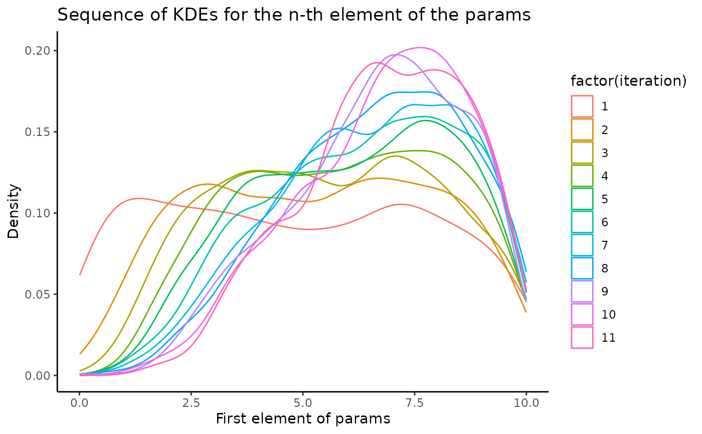
for (col in 1:2) {
  print(col)
  result_matrices_column <- lapply(result_matrices, function(matrix) matrix[, col])


  # create a data frame with one column for the iteration number and one column for the first element of the params
  df <- data.frame(
    iteration = rep(1:length(result_matrices_column), sapply(result_matrices_column, length)),
    params = unlist(result_matrices_column)
  )

  # plot the KDEs
  print(ggplot(df, aes(params, color = factor(iteration))) +
    geom_density(alpha = 0.5) +
    scale_fill_gradient(low = "blue", high = "red") +
    xlab("First element of params") +
    ylab("Density") +
    ggtitle("Sequence of KDEs for the n-th element of the params") +
    theme_classic())
}
#> [1] 1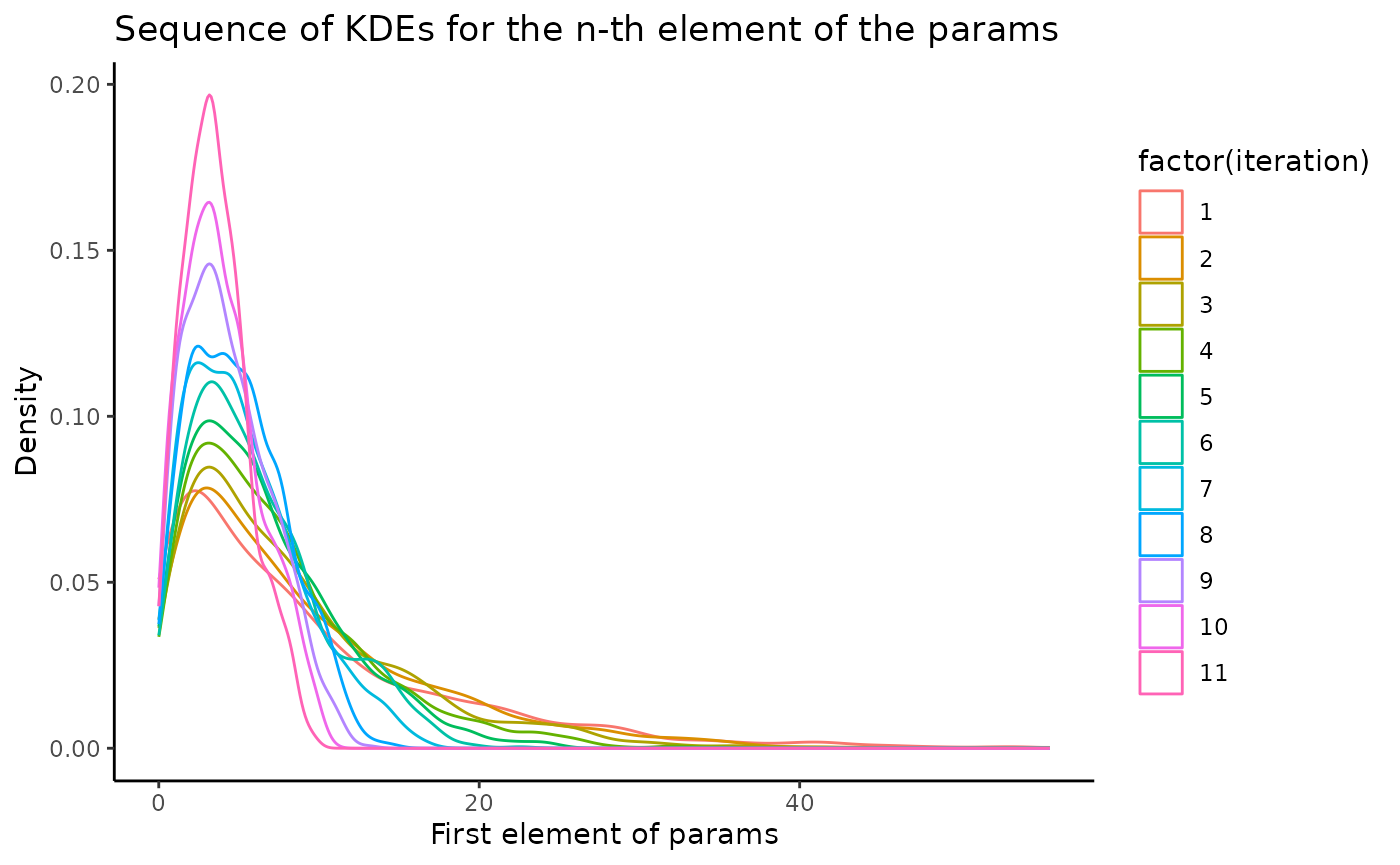

#> [1] 2